IGRF-12

The earth's core behaves as a big magnet. On the surface, we measure different values in magnetic surveys as we move from one geomagnetic pole to the other. The dipole effect of the earth influences all the activities that involves magnetics on earth. This requires us to have a model to predict the earth magnetic flux based on the geographic coordinates of our magnetic surveys.

IGRF-12 means 12th Generation International Geomagnetic Reference Field and it is maintained by The International Association of Geomagnetism and Aeronomy (IAGA). From their official website:

This global main field model provides magnetic field values for any location on Earth, e.g. for navigational purposes (declination) or as a standard for core field subtraction for aeromagnetic surveys. An updated version is adopted by IAGA every 5 years.

Geologist and geophysicist basically gather magnetic data from suveys and subtract the influence of the earth's magnetic field. The result is magnetic information that is caused by the combination of the magnetic susceptibility of all the rocks in the study area.

In this article I will show you how to extract data from the IGRF-12 model using Python.

Tutorial

This tutorial was created in Python 2.7 using Jupyter Notebooks.

Installing requirements

The easiest way to install all the dependencies for this example:

%%bash

conda install -c conda-forge gdal geos geopandas fatiando

Using a Vector File

OPTIONAL - You will only need to do this step if you want to get geomagnetic data inside a vector file. Or maybe plot some geographic info beside the magnetic data.

For this tutorial, we will download the borders of Brazil. I will put it into a directory called data.

%%bash

mkdir data && cd data &&
    wget http://biogeo.ucdavis.edu/data/gadm2.8/gpkg/BRA_adm_gpkg.zip %% # Source: http://www.gadm.org/
    unzip -o BRA_adm_gpkg.zip

Import some modules in Python to visualize the vector file.

geopandas is responsible for integrating pandas with statial data. This is a great module for GIS processing. More information can be found in geopandas docs.

import geopandas as gpd
import matplotlib.pyplot as plt
import numpy as np

%matplotlib inline

brz_df = gpd.GeoSeries.from_file('data/BRA_adm.gpkg')

The Brazil's vector file is too heavy, because the east border is too detailed.

Just for this example I will simplify it using Shapely methods.

brz_df[0] = brz_df[0].simplify(.2).buffer(.05).buffer(-.05)

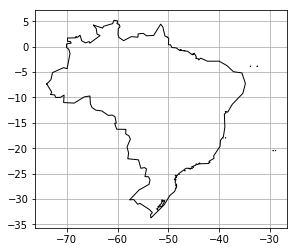
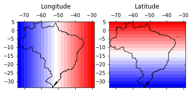
brz_df.plot(alpha=0); plt.grid()

Brazil-1

Preparing the grid

OPTIONAL - If you alread have the coordinates, you don't need to do this unless you want to plot a image.

Get the max and min values of Latitude and Longitude from the .bounds method of the GeoSeries.

lng_min, lat_min, lng_max, lat_max = brz_df.bounds.values.ravel()
extent = [lng_min, lng_max, lat_min, lat_max]

pixel_size = 2

# Subtract the min by the remain of the division of the min by the pixel size.
# ^ This way we get a grid that is multiple of the pixel size. Instead of 1.328631, we get 1.25. Keep Simple!

lng_min = lng_min - (lng_min % pixel_size)
lat_min = lat_min - (lat_min % pixel_size)

Create the range of values from min to max for lats and lngs.

lng_1darray = np.arange(lng_min, lng_max, pixel_size)
lat_1darray = np.arange(lat_max, lat_min, -pixel_size)

Create and visualize a regular grid for the coordinates

lngs, lats = np.meshgrid(lng_1darray, lat_1darray)

fig, axes = plt.subplots(1, 2)
for ax, data, titles in zip(axes.ravel(), [lngs, lats], ['Longitude', 'Latitude']):
    ax.matshow(data, extent=extent, cmap='bwr'); brz_df.plot(alpha=0, ax=ax); ax.set_title(titles, y=1.15)

Brazil-2

Now we need to match the pairs of lngs and lats for each pixel (or cell) of the 2D grid. We do this by changing both to 1d arrays.

They will always match each other after reshaping for 1D if they had the same shape when they were 2D.

lngs.shape == lats.shape

True

shape = lngs.shape
shape

(20, 23)

Extracting data from IGRF-12

Download this script. This was originally a fortran script that I used f2py on it, so we can import into python now. This is based on the professor Michael Hirsch solution called pyigrf12. I automated everything in the cell bellow, but you can download it and put in the same folder of your own python script and import it using import igrf.

You can read the original fortran script for more info, but basically this is a script that does all the computations for the IGRF-12 model. I didn't looked further, but, apparently, is provided by the BGS on top of the coefficients published by the IAGA in 2014.

%%bash

mkdir igrf12 && cd igrf12 && cat > __init__.py &&
    wget http://geologyandpython.com/scripts/igrf.so

Test to see if the script is working:

from igrf12 import igrf

Import numpy, matplotlib and fatiando:

import numpy as np
import matplotlib.pyplot as plt
from fatiando.utils import vec2ang

%matplotlib inline

Your list of coordinates is defined here:

lat = lats.ravel()
lng = lngs.ravel()

Transform latitudes and longitudes into colatitudes and east-longitude:

colat = 90 - lat
elon = (360 + lng) % 360

We are going to call, from Python, the Fortran subroutine called igrf12syn.

For this, need to define some variables (isv, date, itype, alt).

These variables can be found inside the original fortran script's description:

      subroutine igrf12syn (isv,date,itype,alt,colat,elong,x,y,z,f)
c
c     This is a synthesis routine for the 12th generation IGRF as agreed 
c     in December 2014 by IAGA Working Group V-MOD. It is valid 1900.0 to
c     2020.0 inclusive. Values for dates from 1945.0 to 2010.0 inclusive are 
c     definitive, otherwise they are non-definitive.
c   INPUT
c     isv   = 0 if main-field values are required
c     isv   = 1 if secular variation values are required
c     date  = year A.D. Must be greater than or equal to 1900.0 and 
c             less than or equal to 2025.0. Warning message is given 
c             for dates greater than 2020.0. Must be double precision.
c     itype = 1 if geodetic (spheroid)
c     itype = 2 if geocentric (sphere)
c     alt   = height in km above sea level if itype = 1
c           = distance from centre of Earth in km if itype = 2 (>3485 km)
c     colat = colatitude (0-180)
c     elong = east-longitude (0-360)
c     alt, colat and elong must be double precision.
c   OUTPUT
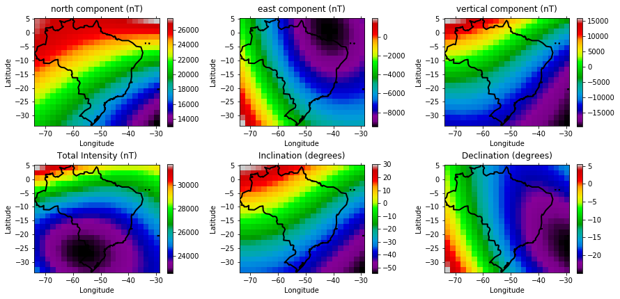
c     x     = north component (nT) if isv = 0, nT/year if isv = 1
c     y     = east component (nT) if isv = 0, nT/year if isv = 1
c     z     = vertical component (nT) if isv = 0, nT/year if isv = 1
c     f     = total intensity (nT) if isv = 0, rubbish if isv = 1

Alright, now we define isv, date, itype, alt. Then create some empty arrays and for each pair of colatitude and east-longitude we call the igrf12syn function.

isv = 0
date = 2010.0
itype = 1
alt = 0.15

x = np.empty_like(colat)
y = np.empty_like(colat)
z = np.empty_like(colat)
f = np.empty_like(colat)
intensity = np.empty_like(colat)
I = np.empty_like(colat)
D = np.empty_like(colat)

for i in np.arange(colat.shape[0]):
    x[i], y[i], z[i], f[i] = igrf.igrf12syn(isv, date, itype, alt, colat[i], elon[i])
    intensity[i], I[i], D[i] = vec2ang([x[i], y[i], z[i]])

Visualizing the arrays

fig, axes = plt.subplots(2, 3, figsize=(12.5, 6))
for ax, data, titles in zip(axes.ravel(),
                            [arr.reshape(shape) for arr in [x, y, z, f, I, D]],
                            ['north component (nT)', 'east component (nT)', 'vertical component (nT)',
                             'Total Intensity (nT)','Inclination (degrees)', 'Declination (degrees)']):

    cax = ax.matshow(data, extent=extent, cmap='spectral') 

    ax.set_title(titles, y=1.02)
    ax.tick_params(labelbottom=True, labeltop=False)
    ax.set_xlabel('Longitude') 
    ax.set_ylabel('Latitude')
    plt.colorbar(cax, ax=ax)

    brz_df.plot(alpha=0, linewidth=2, ax=ax)

fig.tight_layout()

Brazil-Geomag

Get the notebook and try it out

IGRF-12 with Python - Notebook

If you are making use of our methods, please consider donating. The button is at the bottom of the page.

Geology and Python

Extracting geomagnetic data from IGRF-12 with Python