Most part of the earth data is referenced to models (datums) and are unprojected. There are different datums and some of these fit better for a specific part of the earth while other don't. These models exist to approach the shape and size of the earth and make easier for us to locate ourselves on the earth surface. To avoid confusion, let's quote:

From the Intergovernmental Committee on Surveying and Mapping (ICSM):

A datum is a system which allows the location of latitudes and longitudes (and heights) to be identified onto the surface of the Earth - ie onto the surface of a ’round’ object. The basic mathematical/geometric principle which is used is that:

mathematically a ’round’ surface (a modified sphere) is created which represents the surface of the Earth

from here calculations are made to fit this mathematical model to the surface of the Earth - firstly the Equator, then North and South Poles and then lines of latitude and longitude.

Because there are different ways to fit the mathematical model to the surface of the Earth, there are many different datums. Also, in the modern digital era, techniques have vastly improved and many modern datum are very similar to each other. However, also in this modern digital era, people like to know locations precisely so even a small difference may be significant.

Also,

A projection is a process which uses the latitude and longitude which has already been ‘drawn’ on the surface of the Earth using a datum, to then be ‘drawn’ onto a ‘flat piece of paper’ - called a map. See the section on Projections for more information about projection methodologies.

For more information, read the ICSM's Fundamentals of Mapping

There are also some detailed YouTube videos on this. Like this one:

For the good of it's community, Python have some simple solutions for us to do transformation between datums and a easy module to plot using different map projections. We explore these in this article.

Tutorial

This tutorial was created in Python 2.7 using Jupyter Notebooks.

The easiest way to install all the dependencies for this example:

%%bash
conda install -c conda-forge gdal geos pyproj shapely cartopy
pip install overpass

Or you can simply use the geoscience-notebook solution described at the bottom of the Docker article.

Getting data

OPTIONAL: If you already have a list of coordinates, there is no need to do this step.

For this example I will use the Overpass API to extract all major cities in Portugal from the OpenStreetMaps project.

The Overpass API is a read-only API that serves up custom selected parts of the OSM map data. It acts as a database over the web: the client sends a query to the API and gets back the data set that corresponds to the query.

Also,

(...) these coordinates are specified in the OSM database and in the OverPass API by vertically projecting the real points to nodes on the WGS84 ellipsoid.

Let's import some Python modules we are going to use:

import numpy as np
from shapely import geometry
import overpass
import pyproj

The Overpass API query system is a bit complicated. Here is the description of the Query Language: Overpass API Query Language.

Let's call the API object and do a query:

api = overpass.API()
response = api.Get('area[name="Portugal"];(node[place="city"](area););out;')

The response is a Python dictionary containing the data.

Let's use Python's list comprehension to extract the coordinates and names of the cities.

Lists comprehensions provide a concise way to create lists. Common applications are to make new lists where each element is the result of some operations applied to each member of another sequence or iterable, or to create a subsequence of those elements that satisfy a certain condition.

geometry.shape is a shapely method to get a geometry description inside a dictionary and transform it into a shapely object. Then, we call the method .xy to get the actual coordinates.

You can break this cell into steps to understand it better (this is how I learned Python).

names = [city['properties']['name'] for city in response['features']]
coords = [geometry.shape(city['geometry']).xy for city in response['features']]

names is a list containing the city names. Let's check it out:

print u' - '.join(names)

Viseu - Braga - Évora - Vila Real - Setúbal - Portalegre - Santarém - Leiria - Bragança - Faro - Angra do Heroísmo - Funchal - Ponta Delgada - Horta - Nazaré - Marinha Grande - Coimbra - Beja - Lisboa - Castelo Branco - Guarda - Aveiro - Alcobaça - Porto - Viseu - Braga - Évora - Vila Real - Setúbal - Portalegre - Santarém - Leiria - Bragança - Faro - Angra do Heroísmo - Funchal - Ponta Delgada - Horta - Nazaré - Marinha Grande - Coimbra - Beja - Lisboa - Castelo Branco - Guarda - Aveiro - Alcobaça - Porto

coords is a list containing pairs of coordinates. Let's check the first entry of the list:

coords[0]

(array('d', [-7.9138664]), array('d', [40.6574713]))

Here, we call numpy's hstack to do a horizontal stack on the coords object. This way we are stacking longitudes and latitudes into different 1d arrays.

lng, lat = np.hstack(coords)

Coordinate transformation

This examples will first show you how to transform from the World Geodetic System 1984 (WGS84) to the old European Datum 1950 (ED50). These two datums are based on two different ellipsoids.

To transform lats and longs in WGS84 to ED50 we will use pyproj and the EPSG spatial reference list.

pyproj is a Python interface to PROJ4 library for cartographic transformations.

The EPSG Geodetic Parameter Dataset Registry stores geodetic parameters as entities. The Registry maintains lifecycle information for each entity and manages releases of the entire dataset.

pyproj is a easy to use package and is the most simple solution for this in Python. Let's go ahead and transform the coordinates using the datum name for the WGS84 and the EPSG code for the ED50. On both we use geographic unprojected data. The EPSG code is extracted using the http://www.epsg-registry.org site by searching for the name of the datum.

# Define the two projections.
p1 = pyproj.Proj(proj='latlong', datum='WGS84')
p2 = pyproj.Proj(init='epsg:4230')
# Call the tranform method and store the tranformed variables
lng2, lat2 = pyproj.transform(p1, p2, lng, lat)

Let's check the changes of the first 10 tranformations:

for x1, y1, x2, y2 in zip(lng, lat, lng2, lat2)[:10]:
    print '{}, {} ----> {}, {}'.format(x1, y1, x2, y2)

-7.9138664, 40.6574713 ----> -7.91257700014, 40.6586844007
-8.4280045, 41.5510583 ----> -8.42668973799, 41.5522617727
-7.9092808, 38.5707742 ----> -7.90802961104, 38.5720199811
-7.74678, 41.2966556 ----> -7.74548062967, 41.2978558234
-8.8926172, 38.524321 ----> -8.8913526948, 38.5255780146
-7.433342, 39.2911275 ----> -7.43208513376, 39.2923573745
-8.6867081, 39.2363637 ----> -8.68543386742, 39.2376080315
-8.8080365, 39.7445357 ----> -8.8067512015, 39.7457735633
-6.7589839, 41.8071182 ----> -6.75768960546, 41.8082981083
-7.9351771, 37.0162727 ----> -7.93395148636, 37.0175400003

Coordinate transform from WGS84 latlong to the WGS84 UTM coordinates:

# Define the two projections.
p1 = pyproj.Proj(proj='latlong', datum='WGS84')
# You can also search for UTM projections in the epsg reference website
p3 = pyproj.Proj(proj='utm', zone=29, datum='WGS84') 
# Call the tranform method and store the tranformed variables
e, n = pyproj.transform(p1, p3, lng, lat)

Since Portugal have some islands that are far to the west and the UTM representation will add a lot of distortion on those, you may want to filter those values out.

Let's check the transformation:

for x1, y1, x2, y2 in zip(lng, lat, e, n)[:10]:
    print '{}, {} ----> {}, {}'.format(x1, y1, x2, y2)

-7.9138664, 40.6574713 ----> 591817.588662, 4501301.31149
-8.4280045, 41.5510583 ----> 547702.909553, 4600090.63784
-7.9092808, 38.5707742 ----> 595016.547696, 4269710.60289
-7.74678, 41.2966556 ----> 604924.835614, 4572446.86515
-8.8926172, 38.524321 ----> 509360.403574, 4263997.59189
-7.433342, 39.2911275 ----> 635105.354038, 4350253.99166
-8.6867081, 39.2363637 ----> 527038.032027, 4343053.40745
-8.8080365, 39.7445357 ----> 516446.851608, 4399421.42235
-6.7589839, 41.8071182 ----> 686160.41259, 4630788.75125
-7.9351771, 37.0162727 ----> 594725.074546, 4097207.51884

It's that simple! pyproj (and PROJ4) is powerful enough to do bulk coordinate transformations using just 3 lines of code.

Coordinate transform from WGS84 UTM to WGS84 latlong coordinates:

p1 = pyproj.Proj(proj='latlong', datum='WGS84')
p3 = pyproj.Proj(proj='utm', zone=29, datum='WGS84') 
# Notice that we just inverted the projections:
lng, lat = pyproj.transform(p3, p1, e, n)

for x1, y1, x2, y2 in zip(e, n, lng, lat)[:10]:
    print '{}, {} ----> {}, {}'.format(x1, y1, x2, y2)

591817.588662, 4501301.31149 ----> -7.9138664, 40.6574713
547702.909553, 4600090.63784 ----> -8.4280045, 41.5510583
595016.547696, 4269710.60289 ----> -7.9092808, 38.5707742
604924.835614, 4572446.86515 ----> -7.74678, 41.2966556
509360.403574, 4263997.59189 ----> -8.8926172, 38.524321
635105.354038, 4350253.99166 ----> -7.433342, 39.2911275
527038.032027, 4343053.40745 ----> -8.6867081, 39.2363637
516446.851608, 4399421.42235 ----> -8.8080365, 39.7445357
686160.41259, 4630788.75125 ----> -6.7589839, 41.8071182
594725.074546, 4097207.51884 ----> -7.9351771, 37.0162727

pyproj have a list of ellipsoids and projections and can be accessed with the methods .pj_ellps and .pj_list, respectively.

Visualizations using common Map Projections

From Cartopy main page:

Cartopy is a Python package designed to make drawing maps for data analysis and visualisation as easy as possible.

Cartopy makes use of the powerful PROJ.4, numpy and shapely libraries and has a simple and intuitive drawing interface to matplotlib for creating publication quality maps.

Some of the key features of cartopy are:

object oriented projection definitions

point, line, vector, polygon and image transformations between projections

integration to expose advanced mapping in matplotlib with a simple and intuitive interface

powerful vector data handling by integrating shapefile reading with Shapely capabilities

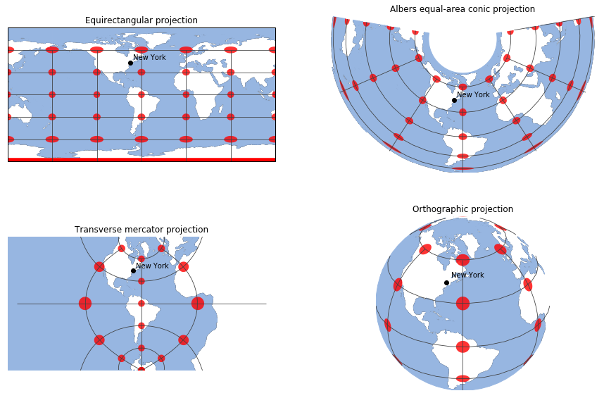
Let's iterate through some map projections and analyse the distortions using the Tissot Indicatrix. And also add a labeled point on the city of New York.

Notice how I added information to the transform argument when I added the point. Everytime a point/line/image is added to a cartopy GeoAxes, it is required to add a coordinate system to the transform of the matplotlib's Axes. I told the Axes that the data is in a Geodetic system, cartopy defaults to the WGS84 datum.

import matplotlib.pyplot as plt
import cartopy.crs as ccrs
from cartopy.feature import OCEAN
import warnings

warnings.filterwarnings('ignore')

projections = [ccrs.PlateCarree(-60), ccrs.AlbersEqualArea(-60), ccrs.TransverseMercator(-60), ccrs.Orthographic(-60, 30)]
titles = ['Equirectangular projection', 
          'Albers equal-area conic projection', 
          'Transverse mercator projection', 
          'Orthographic projection']

fig, axes = plt.subplots(2, 2, subplot_kw={'projection': projections[0]}, figsize=(15,10))

ny_lon, ny_lat = -75, 43

for ax, proj, title in zip(axes.ravel(), projections, titles):
    ax.projection = proj # Here we change projection for each subplot.
    ax.set_title(title) # Add title for each subplot.
    ax.set_global() # Set global extention
    ax.coastlines() # Add coastlines
    ax.add_feature(OCEAN) # Add oceans
    ax.tissot(facecolor='r', alpha=.8, lats=np.arange(-90,90, 30)) # Add tissot indicatrisses
    ax.plot(ny_lon, ny_lat, 'ko', transform=ccrs.Geodetic()) # Plot the point for the NY city
    ax.text(ny_lon + 4, ny_lat + 4, 'New York', transform=ccrs.Geodetic()) # Label New York
    ax.gridlines(color='.25', ylocs=np.arange(-90,90, 30)) # Ad gridlines
plt.show()

4-1

There are some more map projections to be explored in cartopy.crs and tons of customization to do in the maps.

Go ahead and explore the gallery.

Some maps for Portugal

We already have the portuguese cities and their coordinates. So why not create some maps of Portugal?

For this example, I will just filter out the cities located in the western islands. [Longitude > 10° W]

afilter = lng > -10
flng = lng[afilter]
flat = lat[afilter]
fnames = np.asarray(names)[afilter]

Create the extent for the map [xmin, xmax, ymin, ymax].

extent = flng.min() - 1, flng.max() + 1, flat.min() - .5, flat.max() + 1

Create a basemap function. This way we can use it multiple times.

import matplotlib.pyplot as plt
import cartopy.crs as ccrs
from cartopy.feature import BORDERS
from cartopy.io.img_tiles import StamenTerrain
from cartopy.mpl.ticker import LongitudeFormatter, LatitudeFormatter

def basemap_portugal():
    fig = plt.figure(figsize=(10, 10))
    ax = fig.add_subplot(111, projection=ccrs.PlateCarree())
    ax.set_extent(extents=extent, crs=ccrs.Geodetic())
    ax.coastlines(resolution='10m')
    BORDERS.scale = '10m'
    ax.add_feature(BORDERS)

    ax.gridlines(color='.5')
    ax.set_xticks(np.arange(-10, -5, 1), crs=ccrs.PlateCarree())
    ax.set_yticks(np.arange(36, 43, 1), crs=ccrs.PlateCarree())

    ax.xaxis.set_major_formatter(LongitudeFormatter())
    ax.yaxis.set_major_formatter(LatitudeFormatter())
    return fig, ax

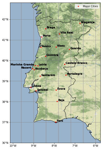
A map with the city names on top of the Stamen Terrain.

fig, ax = basemap_portugal()

ax.plot(flng, flat, 'ro', ms=3, transform=ccrs.Geodetic(),
        label='Major Cities')

for lg, lt, name in zip(flng, flat, fnames):
    if name in [u'Nazaré', 'Marinha Grande']:
        ax.text(lg - .05, lt + .05, 
                name, 
                va='center', 
                ha='right', transform=ccrs.Geodetic(), fontweight='bold')
    else:    
        ax.text(lg + .05, lt + .05, 
                name, 
                va='center', 
                ha='left', transform=ccrs.Geodetic(), fontweight='bold')

st = StamenTerrain()
ax.add_image(st, 8)

ax.legend()

plt.show()

4-2

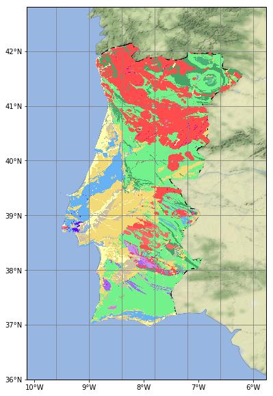
We can also use a WMS service to quickly show the Geologic Units of Portugal. The WMS is provided by the Portuguese Geological Survey to the OneGeology system.

from owslib import wms

def geology_portugal():

    pt_geo = wms.WebMapService(
        'http://geoportal.lneg.pt/arcgis/services/OneGeology/LNEG_EN_Geology/MapServer/WmsServer?')

    fig, ax = basemap_portugal()

    OCEAN.scale = '50m'

    ax.add_feature(OCEAN, color='blue')
    ax.add_feature(BORDERS)

    ax.add_wms(pt_geo, 'OGE_1M_surface_GeologicUnit', zorder=1)
    ax.add_image(st, 7, zorder=0)

    return fig, ax

fig, ax = geology_portugal()
plt.show()

4-3

The legend is provided in this link as an image.

png

Let's crop out the part that we don't want using some Images manipulations in Python.

import urllib, cStringIO
from PIL import Image

URL = 'http://geoportal.lneg.pt/arcgis/services/OneGeology/OGE_CGP1M/MapServer/WMSServer?request=GetLegendGraphic%26version=1.1.1%26format=image/png%26layer=OGE_1M_surface_GeologicUnit'
file = cStringIO.StringIO(urllib.urlopen(URL).read())
img = Image.open(file)

Colors:

colors = img.crop(box=[0, 0, 15, 416])

Labels:

labels = img.crop(box=[233, 0, 442, 416])

Merge colors and labels in a new image:

final_width = colors.width + labels.width
height = colors.height

legend = Image.new('RGB', (final_width, height))
legend.paste(colors, [0, 0, 15, height])
legend.paste(labels, [15, 0, final_width, height])

legend

4-2

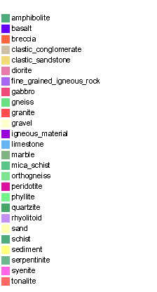
The image resolution of the legend is poor and I'm not sure if it is possible to request a better one to the server.
If this was an image to publish, it would probably be a better idea to recreate the legend instead of cropping and merging it like I did.

Also, cartopy doesn't have a scalebar function yet. But there are some solution out there.

If you are making use of our methods, please consider donating. The button is at the bottom of the page.

Geology and Python

Cartographic Transformation and Map Visualizations in Python

Tutorial

Getting data

Coordinate transformation

Visualizations using common Map Projections

Some maps for Portugal