- 10/01/2018
- Remote-Sensing
- Bruno Ruas de Pinho
- #remote-sensing, #landsat
This post is PART 4 of the Integrating and Exploring series:
- Processing Shapefiles of Lithological Units
- Predicting Spatial Data with Machine Learning
- Download and Process DEMs in Python
- Automated Bulk Downloads of Landsat-8 Data Products in Python
- Fast and Reliable Top of Atmosphere (TOA) calculations of Landsat-8 data in Python
![]()
![]()
Multispectral and hyperspectral satellites are amazing (I'm a huge fan). I tend to think them as a super human vision. Soviet and American space stations started to be launched with multispectral devices in it's equipments in yearly 70's. From them, space scientists have improved it to a solid earth observation system for all kinds of purposes. Today, with these instruments, scientists can accurately categorize trillion of surface pixels, find not only visible, but invisible information, control illegal actions and plan our future as a civilization.
The Landsat Mission is a joint initiative between the U.S. Geological Survey (USGS) and NASA, officially described as:
The world's longest continuously acquired collection of space-based moderate-resolution land remote sensing data.
The Landsat is a multispectral satellite currently on the eighth of it's series. Landsat-8 data is freely available on the USGS's Earth Explorer website. All we need to do is sign up and find a scene that match our area of study. However, in this tutorial, I will show you how to automate the bulk download of low Cloud Covered Landsat-8 images from the comfort your Python!
This is the PART 4 of a series of posts called Integrating & Exploring. This post is also a consequence of the tweet below. Thanks for votes, retweetes and likes!
Which satellite data would you like me to process for the next post? #remotesensing #aster #landsat8 #reflectance
— Geology and Python (@geologynpython) October 28, 2017
Area of Study
Iron River in Michigan, USA
Tutorial
Import pandas and geopandas for easy manipulation and filtering of tables and vector files.folium for interactive map views. os and shutil for file/folder manipulation.
import pandas as pd
import geopandas as gpd
import folium
import os, shutil
from glob import glob
Let's read the vector containing the bounds of the Area of Study. This was processed on previous posts.
bounds = gpd.read_file('./data/processed/area_of_study_bounds.gpkg')
Picking the Best Scenes
The notation used to catalog Landsat-8 images is called Worldwide Reference System 2 (WRS-2). The Landsat follows the same paths imaging the earth every 16 days. Each path is split into multiple rows. So, each scene have a path and a row. 16 days later, another scene will have the same path and row than the previous scene. This is the essence of the WRS-2 system.
USGS provides Shape files of these paths and rows that let us quickly visualize, interact and select the important images.
Let us get the shape files and unpack it. I will first download the file to WRS_PATH and extract it to LANDSAT_PATH.
WRS_PATH = './data/external/Landsat8/wrs2_descending.zip'
LANDSAT_PATH = os.path.dirname(WRS_PATH)

!wget -P {LANDSAT_PATH} https://landsat.usgs.gov/sites/default/files/documents/wrs2_descending.zip

shutil.unpack_archive(WRS_PATH, os.path.join(LANDSAT_PATH, 'wrs2'))
Import it to a GeoDataFrame using geopandas. Check the first 5 entries.
wrs = gpd.GeoDataFrame.from_file('./data/external/Landsat8/wrs2/wrs2_descending.shp')

wrs.head()
| AREA | DAYCLASS | MODE | PATH | PERIMETER | PR | PR_ | PR_ID | RINGS_NOK | RINGS_OK | ROW | SEQUENCE | WRSPR | geometry | |
|---|---|---|---|---|---|---|---|---|---|---|---|---|---|---|
| 0 | 15.74326 | 1 | D | 13 | 26.98611 | 13001 | 1 | 1 | 0 | 1 | 1 | 2233 | 13001 | POLYGON ((-10.80341356392465 80.9888, -8.97406... |
| 1 | 14.55366 | 1 | D | 13 | 25.84254 | 13002 | 2 | 2 | 0 | 1 | 2 | 2234 | 13002 | POLYGON ((-29.24250366707619 80.18681161921363... |
| 2 | 13.37247 | 1 | D | 13 | 24.20303 | 13003 | 3 | 3 | 0 | 1 | 3 | 2235 | 13003 | POLYGON ((-24.04205646041896 79.12261247629547... |
| 3 | 12.26691 | 1 | D | 13 | 22.40265 | 13004 | 4 | 4 | 0 | 1 | 4 | 2236 | 13004 | POLYGON ((-36.66813132081753 77.46094098591608... |
| 4 | 11.26511 | 1 | D | 13 | 20.64284 | 13005 | 5 | 5 | 0 | 1 | 5 | 2237 | 13005 | POLYGON ((-44.11209517917457 76.93655561966702... |
Now, we can check which Polygons of the WRS-2 system intersects with the bounds vector.
wrs_intersection = wrs[wrs.intersects(bounds.geometry[0])]
Also, let's put the calculated paths and rows in a variable.
paths, rows = wrs_intersection['PATH'].values, wrs_intersection['ROW'].values
Create a map to visualize the paths and rows that intersects.
Click on the Polygon to get the path and row value.
# Get the center of the map
xy = np.asarray(bounds.centroid[0].xy).squeeze()
center = list(xy[::-1])

# Select a zoom
zoom = 6

# Create the most basic OSM folium map
m = folium.Map(location=center, zoom_start=zoom, control_scale=True)

# Add the bounds GeoDataFrame in red
m.add_child(folium.GeoJson(bounds.__geo_interface__, name='Area of Study',
                           style_function=lambda x: {'color': 'red', 'alpha': 0}))

# Iterate through each Polygon of paths and rows intersecting the area
for i, row in wrs_intersection.iterrows():
    # Create a string for the name containing the path and row of this Polygon
    name = 'path: %03d, row: %03d' % (row.PATH, row.ROW)
    # Create the folium geometry of this Polygon
    g = folium.GeoJson(row.geometry.__geo_interface__, name=name)
    # Add a folium Popup object with the name string
    g.add_child(folium.Popup(name))
    # Add the object to the map
    g.add_to(m)

folium.LayerControl().add_to(m)
m.save('./images/10/wrs.html')
m
Let's use boolean to remove the paths and rows that intersects just a tiny bit with the area. (paths higher than 26 and lower than 23). This could be done by a threshold of intersection area.
b = (paths > 23) & (paths < 26)
paths = paths[b]
rows = rows[b]
We end up with four pairs of path and row values that would give images covering the area of study.
for i, (path, row) in enumerate(zip(paths, rows)):
    print('Image', i+1, ' - path:', path, 'row:', row)
Image 1  - path: 25 row: 27
Image 2  - path: 25 row: 28
Image 3  - path: 24 row: 28
Image 4  - path: 24 row: 27
Checking Available Images on Amazon S3 & Google Storage
Google and Amazon provides public access to Landsat images.
We can get a DataFrame of available scenes to download in each server using the urls below. The Amazon S3 table has ~20 MB of rows describing the existing data while the Google Storage table has ~500 MB.
s3_scenes = pd.read_csv('http://landsat-pds.s3.amazonaws.com/c1/L8/scene_list.gz', compression='gzip')
# google_scenes = pd.read_csv('https://storage.googleapis.com/gcp-public-data-landsat/index.csv.gz', compression='gzip')
First 3 entries:
s3_scenes.head(3)
| productId | entityId | acquisitionDate | cloudCover | processingLevel | path | row | min_lat | min_lon | max_lat | max_lon | download_url | |
|---|---|---|---|---|---|---|---|---|---|---|---|---|
| 0 | LC08_L1TP_149039_20170411_20170415_01_T1 | LC81490392017101LGN00 | 2017-04-11 05:36:29.349932 | 0.00 | L1TP | 149 | 39 | 29.22165 | 72.41205 | 31.34742 | 74.84666 | https://s3-us-west-2.amazonaws.com/landsat-pds... |
| 1 | LC08_L1TP_012001_20170411_20170415_01_T1 | LC80120012017101LGN00 | 2017-04-11 15:14:40.001201 | 0.15 | L1TP | 12 | 1 | 79.51504 | -22.06995 | 81.90314 | -7.44339 | https://s3-us-west-2.amazonaws.com/landsat-pds... |
| 2 | LC08_L1TP_012002_20170411_20170415_01_T1 | LC80120022017101LGN00 | 2017-04-11 15:15:03.871058 | 0.38 | L1TP | 12 | 2 | 78.74882 | -29.24387 | 81.14549 | -15.04330 | https://s3-us-west-2.amazonaws.com/landsat-pds... |
Now, let's use the previous defined paths and rows intersecting the area and see if there are any available Landsat-8 images in the Amazon S3 storage.
Also, we can select only the images that have a percentage of cloud covering the image less than 5%.
We also want to exclude the product that end with _T2 and _RT, since these are files that must go through calibration and pre-processing. More info!
# Empty list to add the images
bulk_list = []

# Iterate through paths and rows
for path, row in zip(paths, rows):

    print('Path:',path, 'Row:', row)

    # Filter the Landsat Amazon S3 table for images matching path, row, cloudcover and processing state.
    scenes = s3_scenes[(s3_scenes.path == path) & (s3_scenes.row == row) &
                       (s3_scenes.cloudCover <= 5) &
                       (~s3_scenes.productId.str.contains('_T2')) &
                       (~s3_scenes.productId.str.contains('_RT'))]
    print(' Found {} images\n'.format(len(scenes)))

    # If any scenes exists, select the one that have the minimum cloudCover.
    if len(scenes):
        scene = scenes.sort_values('cloudCover').iloc[0]

    # Add the selected scene to the bulk download list.
    bulk_list.append(scene)
Path: 25 Row: 27
 Found 2 images

Path: 25 Row: 28
 Found 6 images

Path: 24 Row: 28
 Found 3 images

Path: 24 Row: 27
 Found 6 images
Check the four images that were selected.
bulk_frame = pd.concat(bulk_list, 1).T
bulk_frame
| productId | entityId | acquisitionDate | cloudCover | processingLevel | path | row | min_lat | min_lon | max_lat | max_lon | download_url | |
|---|---|---|---|---|---|---|---|---|---|---|---|---|
| 679 | LC08_L1TP_025027_20170406_20170414_01_T1 | LC80250272017096LGN00 | 2017-04-06 16:45:24.051124 | 1.51 | L1TP | 25 | 27 | 46.3107 | -91.0755 | 48.4892 | -87.8023 | https://s3-us-west-2.amazonaws.com/landsat-pds... |
| 226329 | LC08_L1TP_025028_20170913_20170928_01_T1 | LC80250282017256LGN00 | 2017-09-13 16:46:22.160327 | 0.06 | L1TP | 25 | 28 | 44.8846 | -91.5385 | 47.0651 | -88.3262 | https://s3-us-west-2.amazonaws.com/landsat-pds... |
| 255166 | LC08_L1TP_024028_20171008_20171023_01_T1 | LC80240282017281LGN00 | 2017-10-08 16:40:21.299100 | 0.23 | L1TP | 24 | 28 | 44.9159 | -89.9783 | 47.0759 | -86.858 | https://s3-us-west-2.amazonaws.com/landsat-pds... |
| 127668 | LC08_L1TP_024027_20170720_20170728_01_T1 | LC80240272017201LGN00 | 2017-07-20 16:39:33.524611 | 3.11 | L1TP | 24 | 27 | 46.3429 | -89.4354 | 48.5005 | -86.2616 | https://s3-us-west-2.amazonaws.com/landsat-pds... |
Last step is to download all files in the server for the 4 images, including metadata and QA. Each product for it's own folder.
# Import requests and beautiful soup
import requests
from bs4 import BeautifulSoup

# For each row
for i, row in bulk_frame.iterrows():

    # Print some the product ID
    print('\n', 'EntityId:', row.productId, '\n')
    print(' Checking content: ', '\n')

    # Request the html text of the download_url from the amazon server.
    # download_url example: https://landsat-pds.s3.amazonaws.com/c1/L8/139/045/LC08_L1TP_139045_20170304_20170316_01_T1/index.html
    response = requests.get(row.download_url)

    # If the response status code is fine (200)
    if response.status_code == 200:

        # Import the html to beautiful soup
        html = BeautifulSoup(response.content, 'html.parser')

        # Create the dir where we will put this image files.
        entity_dir = os.path.join(LANDSAT_PATH, row.productId)
        os.makedirs(entity_dir, exist_ok=True)

        # Second loop: for each band of this image that we find using the html <li> tag
        for li in html.find_all('li'):

            # Get the href tag
            file = li.find_next('a').get('href')

            print('  Downloading: {}'.format(file))

            # Download the files
            # code from: https://stackoverflow.com/a/18043472/5361345

            response = requests.get(row.download_url.replace('index.html', file), stream=True)

            with open(os.path.join(entity_dir, file), 'wb') as output:
                shutil.copyfileobj(response.raw, output)
            del response
EntityId: LC08_L1TP_025027_20170406_20170414_01_T1

 Checking content:

  Downloading: LC08_L1TP_025027_20170406_20170414_01_T1_B9.TIF.ovr
  Downloading: LC08_L1TP_025027_20170406_20170414_01_T1_B11.TIF
  Downloading: LC08_L1TP_025027_20170406_20170414_01_T1_B11.TIF.ovr
  ...
  ...
  ...

  Downloading: LC08_L1TP_025027_20170406_20170414_01_T1_B1.TIF.ovr

EntityId: LC08_L1TP_025028_20170913_20170928_01_T1

  Checking content:

  Downloading: LC08_L1TP_025028_20170913_20170928_01_T1_B4_wrk.IMD
  ...
  ...
  ...
  ...
Let's plot the raw images for the thermal band 10.
import rasterio
from rasterio.transform import from_origin
from rasterio.warp import reproject, Resampling
import matplotlib.pyplot as plt
import cartopy.crs as ccrs
import numpy as np
%matplotlib inline
Read the rasters using rasterio and extract the bounds.
xmin, xmax, ymin, ymax = [], [], [], []

for image_path in glob(os.path.join(LANDSAT_PATH, '*/*B10.TIF')):
    with rasterio.open(image_path) as src_raster:
        xmin.append(src_raster.bounds.left)
        xmax.append(src_raster.bounds.right)
        ymin.append(src_raster.bounds.bottom)
        ymax.append(src_raster.bounds.top)
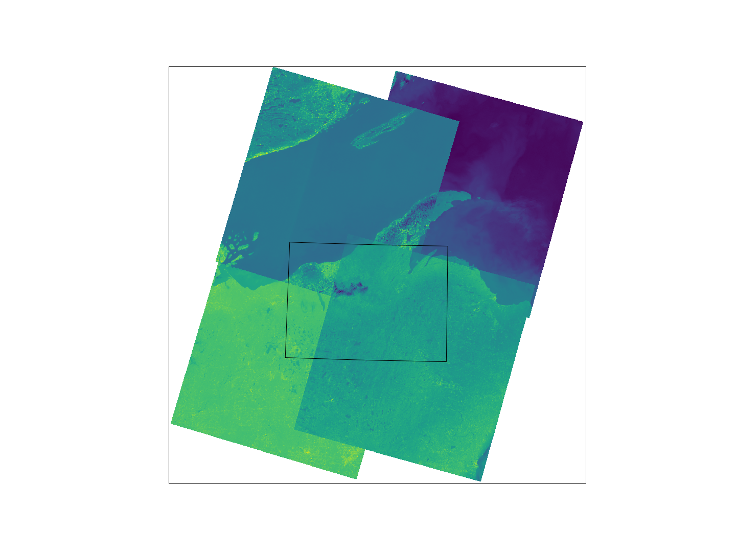
Reproject and plot it.
fig, ax = plt.subplots(1, 1, figsize=(20, 15), subplot_kw={'projection': ccrs.UTM(16)})

ax.set_extent([min(xmin), max(xmax), min(ymin), max(ymax)], ccrs.UTM(16))

bounds.plot(ax=ax, transform=ccrs.PlateCarree())

for image_path in glob(os.path.join(LANDSAT_PATH, '*/*B10.TIF')):

    with rasterio.open(image_path) as src_raster:

        extent = [src_raster.bounds[i] for i in [0, 2, 1, 3]]

        dst_transform = from_origin(src_raster.bounds.left, src_raster.bounds.top, 250, 250)

        width = np.ceil((src_raster.bounds.right - src_raster.bounds.left) / 250.).astype('uint')
        height = np.ceil((src_raster.bounds.top - src_raster.bounds.bottom) / 250.).astype('uint')

        dst = np.zeros((height, width))

        reproject(src_raster.read(1), dst,
                  src_transform=src_raster.transform,
                  dst_transform=dst_transform,
                  resampling=Resampling.nearest)

        ax.matshow(np.ma.masked_equal(dst, 0), extent=extent, transform=ccrs.UTM(16))


fig.savefig('./images/10/landsat.png')
That's it, I download all the images that cover the area of study. Next post, I will go step-by-step on how to derivate the Top of Atmosphere (TOA) reflectance.
Update
LC08_L1TP_025027_20170406_20170414_01_T1 happened to be a very cloudy image. We will have to replace that (palmface).
shutil.rmtree('./data/external/Landsat8/LC08_L1TP_025027_20170406_20170414_01_T1')
Let's check the other scenes available.
scenes = s3_scenes[(s3_scenes.path == 25) & (s3_scenes.row == 27) & (s3_scenes.cloudCover <= 5)]
scenes
| productId | entityId | acquisitionDate | cloudCover | processingLevel | path | row | min_lat | min_lon | max_lat | max_lon | download_url | |
|---|---|---|---|---|---|---|---|---|---|---|---|---|
| 679 | LC08_L1TP_025027_20170406_20170414_01_T1 | LC80250272017096LGN00 | 2017-04-06 16:45:24.051124 | 1.51 | L1TP | 25 | 27 | 46.31065 | -91.07553 | 48.48919 | -87.80226 | https://s3-us-west-2.amazonaws.com/landsat-pds... |
| 151268 | LC08_L1TP_025027_20170812_20170812_01_RT | LC80250272017224LGN00 | 2017-08-12 16:45:54.040574 | 2.75 | L1TP | 25 | 27 | 46.31171 | -91.04313 | 48.49034 | -87.76716 | https://s3-us-west-2.amazonaws.com/landsat-pds... |
| 164949 | LC08_L1TP_025027_20170812_20170824_01_T1 | LC80250272017224LGN00 | 2017-08-12 16:45:54.040574 | 2.75 | L1TP | 25 | 27 | 46.31171 | -91.04313 | 48.49034 | -87.76716 | https://s3-us-west-2.amazonaws.com/landsat-pds... |
Drop using the index of the deleted image and add the new image.
bulk_frame = pd.concat([bulk_frame.drop(679).T, scenes.loc[164949]], axis=1).T
bulk_frame
| productId | entityId | acquisitionDate | cloudCover | processingLevel | path | row | min_lat | min_lon | max_lat | max_lon | download_url | |
|---|---|---|---|---|---|---|---|---|---|---|---|---|
| 226329 | LC08_L1TP_025028_20170913_20170928_01_T1 | LC80250282017256LGN00 | 2017-09-13 16:46:22.160327 | 0.06 | L1TP | 25 | 28 | 44.8846 | -91.5385 | 47.0651 | -88.3262 | https://s3-us-west-2.amazonaws.com/landsat-pds... |
| 127668 | LC08_L1TP_024027_20170720_20170728_01_T1 | LC80240272017201LGN00 | 2017-07-20 16:39:33.524611 | 3.11 | L1TP | 24 | 27 | 46.3429 | -89.4354 | 48.5005 | -86.2616 | https://s3-us-west-2.amazonaws.com/landsat-pds... |
| 255166 | LC08_L1TP_024028_20171008_20171023_01_T1 | LC80240282017281LGN00 | 2017-10-08 16:40:21.299100 | 0.23 | L1TP | 24 | 28 | 44.9159 | -89.9783 | 47.0759 | -86.858 | https://s3-us-west-2.amazonaws.com/landsat-pds... |
| 164949 | LC08_L1TP_025027_20170812_20170824_01_T1 | LC80250272017224LGN00 | 2017-08-12 16:45:54.040574 | 2.75 | L1TP | 25 | 27 | 46.3117 | -91.0431 | 48.4903 | -87.7672 | https://s3-us-west-2.amazonaws.com/landsat-pds... |
Now we can download again using the requests code above.
This post is PART 4 of the Integrating and Exploring series:
- Processing Shapefiles of Lithological Units
- Predicting Spatial Data with Machine Learning
- Download and Process DEMs in Python
- Automated Bulk Downloads of Landsat-8 Data Products in Python
- Fast and Reliable Top of Atmosphere (TOA) calculations of Landsat-8 data in Python