Predicting Spatial Data with Machine Learning

11/09/2017
Machine Learning
Bruno Ruas de Pinho
#geophysics, #data-processing, #machine-learning

This post is PART 2 of the Integrating and Exploring series:

This is the PART 2 of a series of posts called Integrating & Exploring.

In this post, I will preprocess all the magnetic data and predict data on non-sampled using Machine Learning.

Area of Study

Fixed: was referencing wrong dataset

Iron River in Michigan, USA

I choose this specific area because of the presence of Geological, Geophysical and Geochemical data. It will be nice to explore!

Data

All data was downloaded from the USGS - Mineral Resources Online Spatial Data. The data is composed by:

one Geophysics surveys (Magnetic anomaly and Radiometric - in .xyz);
two Geological Maps (WI and MI, USA - in .shp) - processed in PART1;

Geophysics

Title: Airborne geophysical survey: Iron River 1° x 2° Quadrangle

Publication_Date: 2009

Geospatial_Data_Presentation_Form: tabular digital data

Online_Linkage: https://mrdata.usgs.gov/magnetic/show-survey.php?id=NURE-164

Metadata: https://mrdata.usgs.gov/geophysics/surveys/NURE/iron_river/iron_river_meta.html

Beginning Flight Date: 1977 / 04 / 25

Survey height: 400 ft

Flight-line spacing: 3 miles

Tutorial

Let's start by importing some modules.

import pandas as pd
import geopandas as gpd
import numpy as np
import matplotlib.pyplot as plt
from shapely import geometry
import seaborn as sns
%matplotlib inline

Reading files

The code below will check if pycpt is installed and will try to load a nice Colormap for Geophysics plots. If an error occurs, it will use the inverse of the matplotlib's Spectral Colormap.

try:
    import pycpt
    cmap = pycpt.load.cmap_from_cptcity_url('ukmo/wow/temp-c.cpt')
except:
    cmap = 'Spectral_r'

Use seaborn-notebook style for all matplotlib's plots.

plt.style.use('seaborn-notebook')

We already did the coordinate transformation for the magnetic data in the previous post. So let's just import it into pandas, recreate a column for geometry and add it to GeoPandas with spatial information.

mag_data = pd.read_csv('./data/processed/mag.csv', index_col=0)
mag_data['geometry'] = [geometry.Point(x, y) for x, y in zip(mag_data['long_wgs84'], mag_data['lat_wgs84'])]
mag_data = gpd.GeoDataFrame(mag_data, geometry='geometry', crs="+init=epsg:4326")

mag_data.head()

	line	latitude	longitude	totmag	long_wgs84	lat_wgs84	E_utm	N_utm	geometry
0	24	46.0237	-89.9960	59280.2	-89.996159	46.023649	268103.008274	5.101040e+06	POINT (-89.9961587552 46.02364873760001)
1	24	46.0237	-89.9950	59283.0	-89.995159	46.023649	268180.405926	5.101037e+06	POINT (-89.9951587294 46.0236487442)
2	24	46.0237	-89.9944	59283.8	-89.994559	46.023649	268226.844518	5.101036e+06	POINT (-89.99455871399999 46.0236487481)
3	24	46.0237	-89.9934	59281.0	-89.993559	46.023649	268304.242173	5.101033e+06	POINT (-89.9935586882 46.02364875470001)
4	24	46.0237	-89.9928	59276.5	-89.992959	46.023649	268350.680767	5.101031e+06	POINT (-89.9929586727 46.0236487586)

Removing geomagnetic interference

Let's go ahead and do the same thing we did in the IGRF-12 post to get geomagnetic data and subtract the Total Magnetic (totmag) data to get the Residual Magnetic values (resmag).

%%bash

mkdir igrf12 && cd igrf12 && cat > __init__.py &&
    wget http://geologyandpython.com/scripts/igrf.so

from igrf12 import igrf
from fatiando.utils import vec2ang

colat = 90 - mag_data.lat_wgs84
elon = (360 + mag_data.long_wgs84) % 360

isv = 0
date = 1977 + 4.0/12
itype = 1
alt = 400 * 0.3048 / 1000

x = np.empty_like(colat)
y = np.empty_like(colat)
z = np.empty_like(colat)
f = np.empty_like(colat)
intensity = np.empty_like(colat)
I = np.empty_like(colat)
D = np.empty_like(colat)

for i in np.arange(colat.shape[0]):
    x[i], y[i], z[i], f[i] = igrf.igrf12syn(isv, date, itype, alt, colat[i], elon[i])
    intensity[i], I[i], D[i] = vec2ang([x[i], y[i], z[i]])

mag_data['resmag_igrf12'] = mag_data.totmag - f
resmag = mag_data['resmag_igrf12']

Let's check the distribution plot of the resmag using seaborn.

ax = sns.distplot(resmag, axlabel='Residual magnetic value (nT)')
ax.get_figure().savefig('images/7/1.png')

7-1

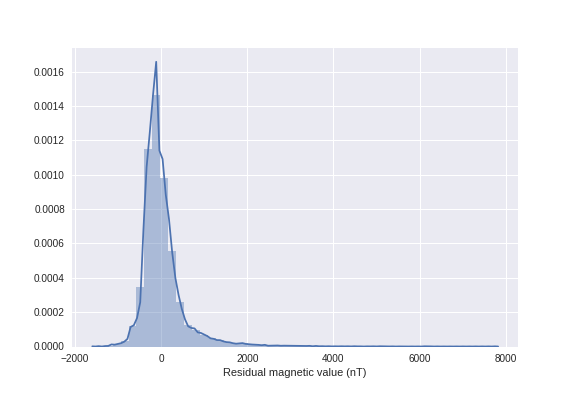
It seems that we have some outliers. Let's switch the data over 98% and under 0.1% of the quantile to NaNs (I did some iterations here to find these values).

resmag.loc[resmag < resmag.quantile(.001)] = np.nan
resmag.loc[resmag > resmag.quantile(.98)] = np.nan

/opt/conda/envs/python2/lib/python2.7/site-packages/pandas/core/indexing.py:179: SettingWithCopyWarning: 
A value is trying to be set on a copy of a slice from a DataFrame

See the caveats in the documentation: http://pandas.pydata.org/pandas-docs/stable/indexing.html#indexing-view-versus-copy
  self._setitem_with_indexer(indexer, value)

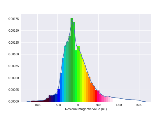
Define the minimun and maximun values for the Colormap.

vmin = -750
vmax = 900

Let's check how these values go:

ax = sns.distplot(mag_data.resmag_igrf12.dropna(), axlabel='Residual magnetic value (nT)')
[patch.set_color(cmap(plt.Normalize(vmin=vmin, vmax=vmax)(patch.xy[0]))) for patch in ax.patches]
[patch.set_alpha(1) for patch in ax.patches]
ax.get_figure().savefig('images/7/2.png')

7-2

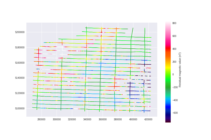
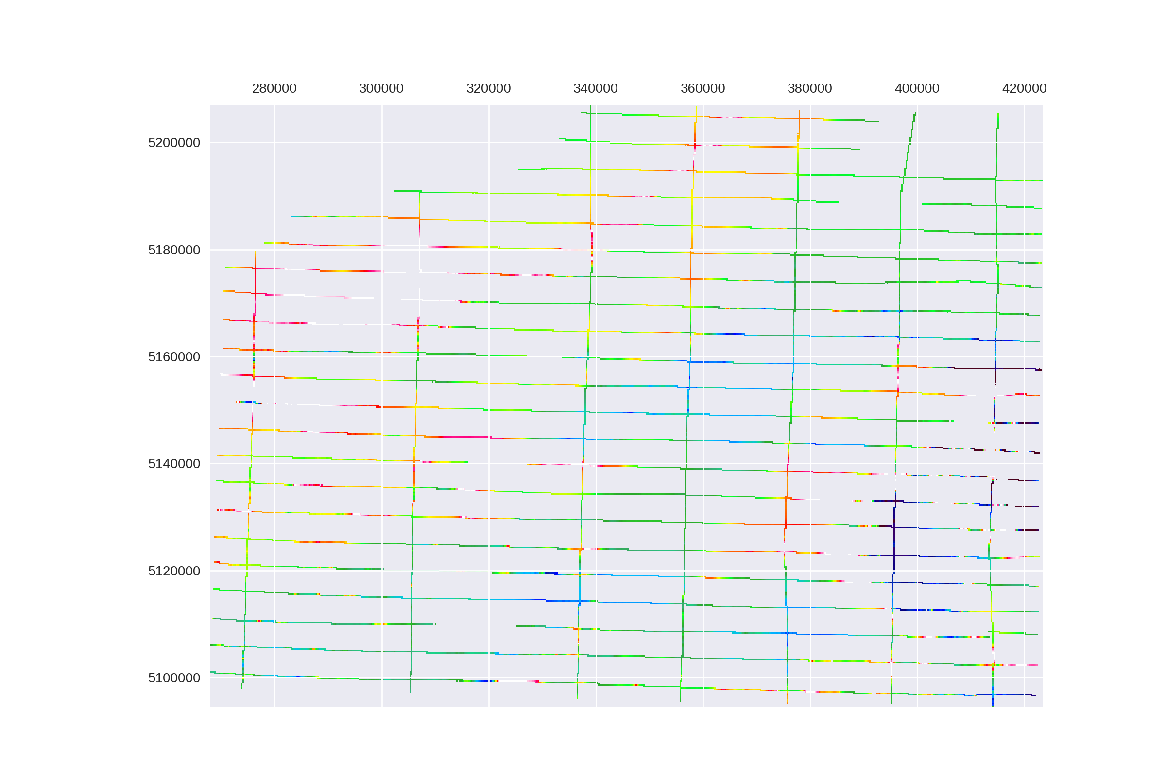
Alright, use plt.scatter to quickly visualize our flight lines with these colors (don't do this for bigger datasets)

plt.scatter(mag_data.E_utm, mag_data.N_utm, cmap=cmap, s=1, c=resmag, vmin=vmin, vmax=vmax)
plt.colorbar(label=u'Residual magnetic value (nT)')
plt.gca().set_aspect('equal')
plt.gcf().set_size_inches(12, 8)
plt.savefig('images/7/3.png')

7-3

Creating a Numpy Array to allocate the predicted data

Now we need to create a array that encompasses all the survey readings.

Defining the pixel size (I'm not sure if there is an ideal value here, leave a comment if you have some more info on this).

pixel_size = 250

Now, define the range of coordinate values to be processed as a function to the pixel size.

x_range = np.arange(mag_data.E_utm.min() - mag_data.E_utm.min() % pixel_size,
                    mag_data.E_utm.max(), pixel_size)
y_range = np.arange(mag_data.N_utm.min() - mag_data.N_utm.min() % pixel_size,
                    mag_data.N_utm.max(), pixel_size)[::-1]

Define the shape.

shape = (len(y_range), len(x_range))

Define the extent.

extent = xmin, xmax, ymin, ymax = x_range.min(), x_range.max(), y_range.min(), y_range.max()

Check the information we just added.

print '''Array info:
rows: {}, columns: {}\nxmin: {}, xmax: {}\nymin: {}, ymax: {}
'''.format(shape[0], shape[1], xmin, xmax, ymin, ymax)

Array info:
rows: 451, columns: 623
xmin: 268000.0, xmax: 423500.0
ymin: 5094500.0, ymax: 5207000.0

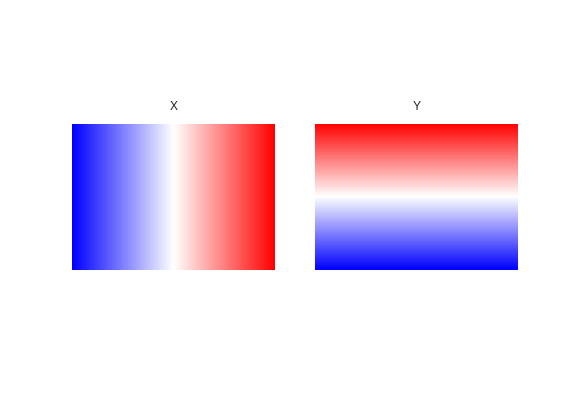
From the ranges, let's call meshgrid to get the coordinates in 2D arrays.

x_mesh, y_mesh = np.meshgrid(x_range, y_range)

Check if its correct:

fig, axes = plt.subplots(1, 2)
for ax, data, title in zip(axes.ravel(), [x_mesh, y_mesh], ['X', 'Y']):
    ax.matshow(data, extent=extent, cmap='bwr'); ax.set_axis_off(); ax.set_title(title)
fig.savefig('images/7/4.png')

7-4

Now that we have defined a array. We can convert each sample's UTM coordinate to index values of the array.

mag_data.loc[:, 'X_INDEX'] = ((mag_data.E_utm - xmin) / pixel_size).astype(int)
mag_data.loc[:, 'Y_INDEX'] = (shape[0] - ((mag_data.N_utm - ymin) / pixel_size)).astype(int)

Create an empty array with the shape that we defined previously and add the resmag values into the positions defined by the index.

mag_array = np.zeros(shape)
mag_array[:] = np.nan
mag_array[mag_data.Y_INDEX, mag_data.X_INDEX] = resmag

Let's check if the gridded values are in (or at least very close to) their original place.

plt.matshow(mag_array, cmap=cmap, vmin=vmin, vmax=vmax, extent=extent)
plt.gcf().set_size_inches(12, 8)
plt.gcf().set_dpi(200)
plt.savefig('images/7/5.png')

7-5

Machine Learning to Predict Spatial Data

Machine Learning (ML) methods can be used for fast solutions of complex problems, like spatial data prediction!

I will use the scikit-learn python module for Machine Learning. From http://scikit-learn.org:

scikit-learn

Machine Learning in Python

Simple and efficient tools for data mining and data analysis

Accessible to everybody, and reusable in various contexts

Built on NumPy, SciPy, and matplotlib

Open source, commercially usable - BSD license

In this part of the code, I will quick check which algorithms will provide better visual results for this prediction problem.

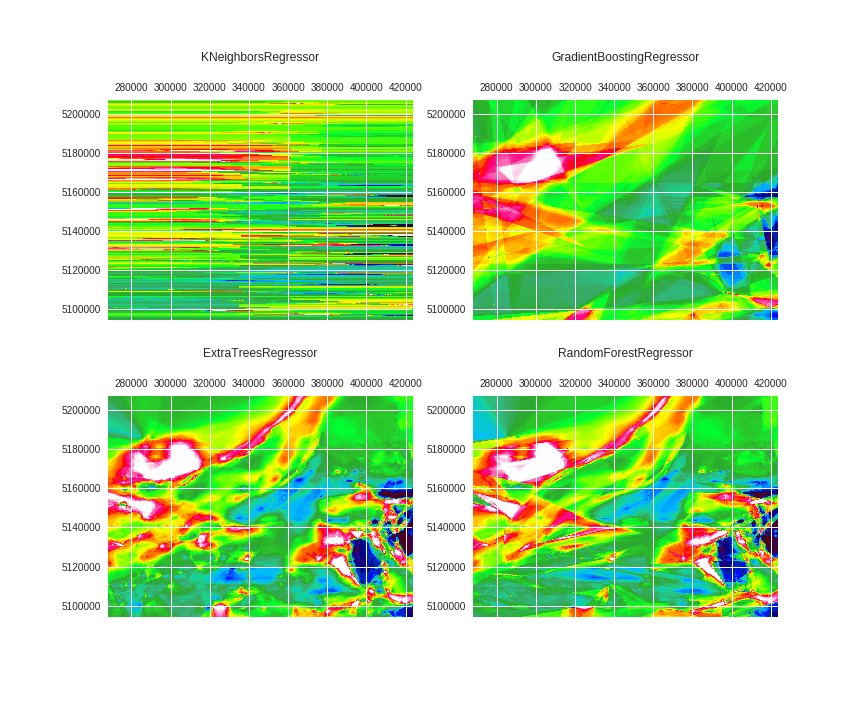
Let's check four different Machine Learning algorithms to predict using only EAST and NORTH coordinates as features.

from sklearn.ensemble import RandomForestRegressor, ExtraTreesRegressor, GradientBoostingRegressor
from sklearn.neighbors import KNeighborsRegressor
from sklearn.preprocessing import MinMaxScaler

regrs = [KNeighborsRegressor(),
        GradientBoostingRegressor(),
        ExtraTreesRegressor(),
        RandomForestRegressor()
       ]

y_fit = mag_array[np.isfinite(mag_array)]
x_index_fit, y_index_fit = np.where(np.isfinite(mag_array))
x_index_pred, y_index_pred = np.where(mag_array)

X_fit = MinMaxScaler().fit_transform(np.vstack([x_index_fit, y_index_fit]).T)
X_pred = MinMaxScaler().fit_transform(np.vstack([x_index_pred, y_index_pred]).T)

fig, axes = plt.subplots(2, 2, figsize=(12,10))
for ax, regr, title in zip(axes.ravel(),
                          regrs,
                          ['KNeighborsRegressor', 
                           'GradientBoostingRegressor', 
                           'ExtraTreesRegressor', 
                           'RandomForestRegressor']):

    regr.fit(X=X_fit, y=y_fit)
    y_pred = regr.predict(X=X_pred)

    ax.matshow(y_pred.reshape(shape), extent=extent, cmap=cmap, vmin=vmin, vmax=vmax)
    ax.set_title(title, y=1.15)
fig.savefig('images/7/6.png')

7-6

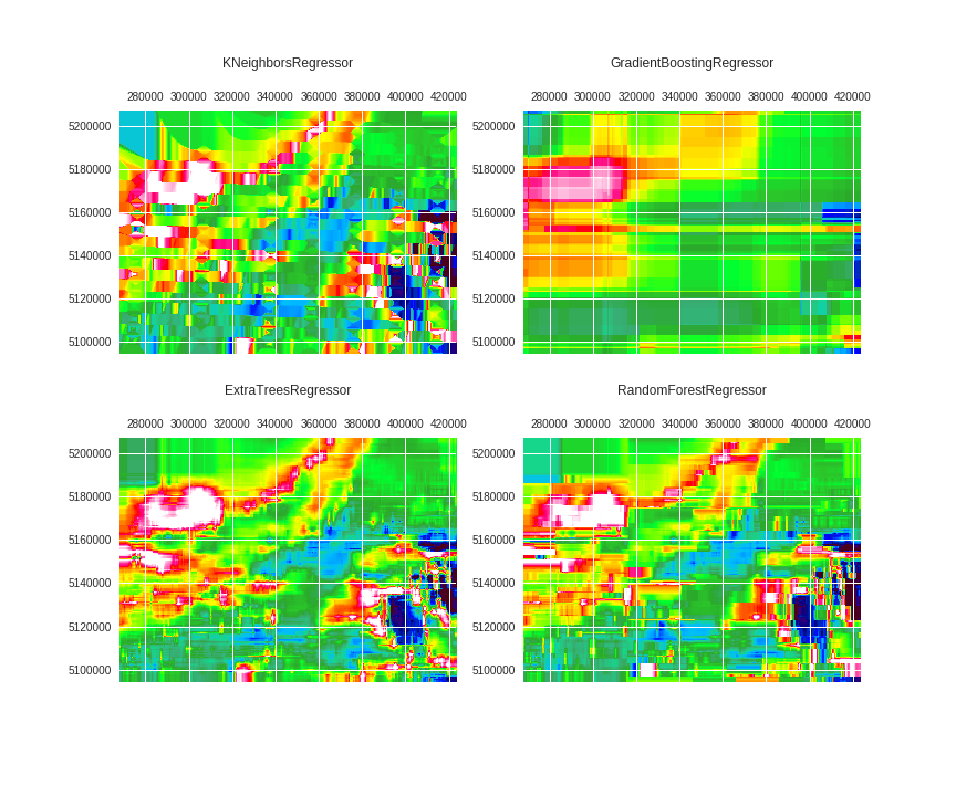
yuck! It was trained using only two directions (east and north). What if we rotate it? Would the algorithm learn spatial continuity in all directions?

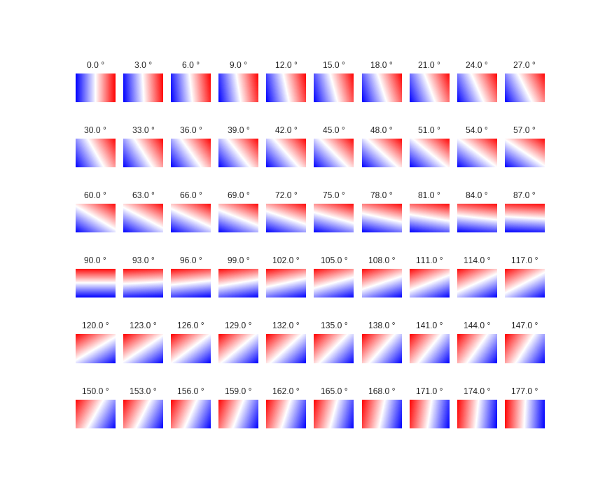
Adding complexity to the X, Y data

Let's add complexity to our features by rotating the array. This works, the same way complexity is added with PolynomialFeatures:

n_angles = 60

X_var, Y_var, angle = np.meshgrid(x_range, y_range, n_angles)

angles = np.deg2rad(np.linspace(0, 180, n_angles, endpoint=False))

X = X_var + np.tan(angles) * Y_var
X[:,:,(n_angles/2)+1:] = np.flipud(np.fliplr(X[:,:,(n_angles/2)+1:]))

fig, axes = plt.subplots(6, 10, figsize=(12, 10))
for ax, data, angle in zip(axes.ravel(), np.dsplit(X, 60), angles):
    ax.matshow(data.squeeze(), extent=extent, cmap='bwr'); ax.set_axis_off()
    ax.set_title(u'{} °'.format(str(np.rad2deg(angle))))
fig.savefig('images/7/7.png')

7-7

Finally, sample the rotated arrays and train the Regressors:

X_fit = X[x_index_fit, y_index_fit]

X_pred = X.reshape(-1, 60)
preds = dict()
fig, axes = plt.subplots(2, 2, figsize=(12,10))
for ax, regr, title in zip(axes.ravel(),
                          regrs,
                            ['KNeighborsRegressor',
                             'GradientBoostingRegressor', 
                             'ExtraTreesRegressor', 
                             'RandomForestRegressor']):

    regr.fit(X=X_fit, y=y_fit)
    y_pred = regr.predict(X=X_pred)
    preds[title] = y_pred
    ax.matshow(y_pred.reshape(shape), extent=extent, cmap=cmap, vmin=vmin, vmax=vmax)
    ax.set_title(title, y=1.15)
fig.savefig('images/7/8.png')

7-8

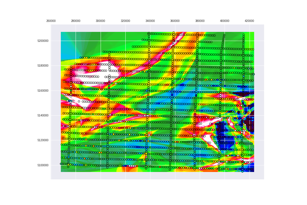
Let's check the results for the RandomForestRegressor and ExtraTreesRegressor.

mag_RF = preds['RandomForestRegressor'].reshape(shape)
mag_ETF = preds['ExtraTreesRegressor'].reshape(shape)

Here we add the known values on top of the predicted values.

fig = plt.figure(figsize=(15, 10))
ax = fig.add_subplot(111)
ax.matshow(mag_RF, extent=extent, cmap=cmap, vmin=vmin, vmax=vmax)
ax.scatter(mag_data.E_utm[::25], mag_data.N_utm[::25], 
           cmap=cmap, s=40, c=resmag[::25], vmin=vmin, vmax=vmax, linewidths=1, edgecolors='k')
fig.savefig('images/7/9.png')

7-9

Let's check the ExtraTreesRegressor predictions on top of the USGS geology for the Area of Study, from PART1.

geology = gpd.read_file('./data/processed/geology/geology.shp')

fig = plt.figure(figsize=(15, 10))
ax = fig.add_subplot(111)
ax.matshow(mag_ETF, extent=extent, cmap=cmap, vmin=vmin, vmax=vmax)
geology.to_crs({'init': 'epsg:32616'}).plot(alpha=0, ax=ax, edgecolor='.25')
fig.savefig('images/7/10.png')

7-10

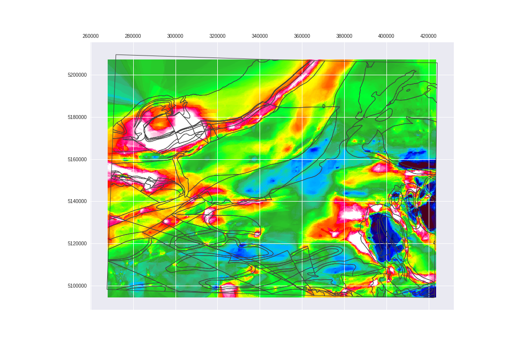
Nice! BUT It is not that simple...

Notice that although this model seems to be doing decent predictions it is overfitted to the dataset, because the entire dataset was used to train the model. This is wrong and should be avoided.

To overpass this problem, we split the known values into train , test and validation datasets before starting the training pipeline. This is called cross validation.

One can also search for the best parameters for each Regression Model as a function of a specific dataset. This is called hyper-parameter tunning.

Do we geoscientists have to care about all these stuff?

Not really! Keep reading.

Automated Machine Learning (AutoML)

AutoML is basically a technic to automate all the process of model selection, hyper-parameter tuning and cross-validation to get the best model for a dataset.

In Python, I use tpot

Consider TPOT your Data Science Assistant. TPOT is a Python Automated Machine Learning tool that optimizes machine learning pipelines using genetic programming.

There is also auto-sklearn for completing the same tasks.

Choose one and start training machines to train machines to train machines...

import tpot

tregr = tpot.TPOTRegressor(n_jobs=7, verbosity=2, generations=5, warm_start=True)

Fit data. This will look into all the available models for our data:

tregr.fit(X_fit, y_fit)

Optimization Progress:  30%|██▉       | 177/600 [25:21<3:16:37, 27.89s/pipeline]

Generation 1 - Current best internal CV score: 107604.750247

TPOT closed prematurely. Will use the current best pipeline.

Best pipeline: ExtraTreesRegressor(input_matrix, ExtraTreesRegressor__bootstrap=False, ExtraTreesRegressor__max_features=DEFAULT, ExtraTreesRegressor__min_samples_leaf=19, ExtraTreesRegressor__min_samples_split=8, ExtraTreesRegressor__n_estimators=100)

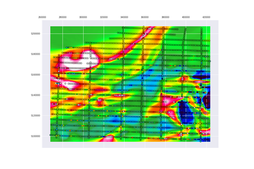
I interrupted it early and I ended up with a fair model to predict the dataset:

AutoML is made to be running for a veeeery long time. The more it searches, better are the predictions made by the models. Keep reading about AutoML.

Let's predict:

tpot_pred = tregr.predict(X_pred)
mag_TPOT = tpot_pred.reshape(shape)

Save the model:

tregr.export('models/spatial_interpolator.py')

And visualize the predictions:

fig = plt.figure(figsize=(15, 10))
ax = fig.add_subplot(111)
ax.matshow(mag_TPOT, extent=extent, cmap=cmap, vmin=vmin, vmax=vmax)
ax.scatter(mag_data.E_utm[::25], mag_data.N_utm[::25], 
           cmap=cmap, s=40, c=resmag[::25], vmin=vmin, vmax=vmax, linewidths=1, edgecolors='k')
plt.savefig('images/7/11.png')

7-11

It is also possible to reduce the amount of models that TPOT will do the search in so it will skip the algorithms that we are not interested in, like: KNeighborsRegressor and GradientBoostingRegressor.

Let's add a hillshade layers to improve the visualization of the magnetic units.

This hillshade function is from the GeoExamples blog:

def hillshade(array, azimuth, angle_altitude):

    # Source: http://geoexamples.blogspot.com.br/2014/03/shaded-relief-images-using-gdal-python.html

    x, y = np.gradient(array)
    slope = np.pi/2. - np.arctan(np.sqrt(x*x + y*y))
    aspect = np.arctan2(-x, y)
    azimuthrad = azimuth*np.pi / 180.
    altituderad = angle_altitude*np.pi / 180.


    shaded = np.sin(altituderad) * np.sin(slope)\
     + np.cos(altituderad) * np.cos(slope)\
     * np.cos(azimuthrad - aspect)
    return 255*(shaded + 1)/2

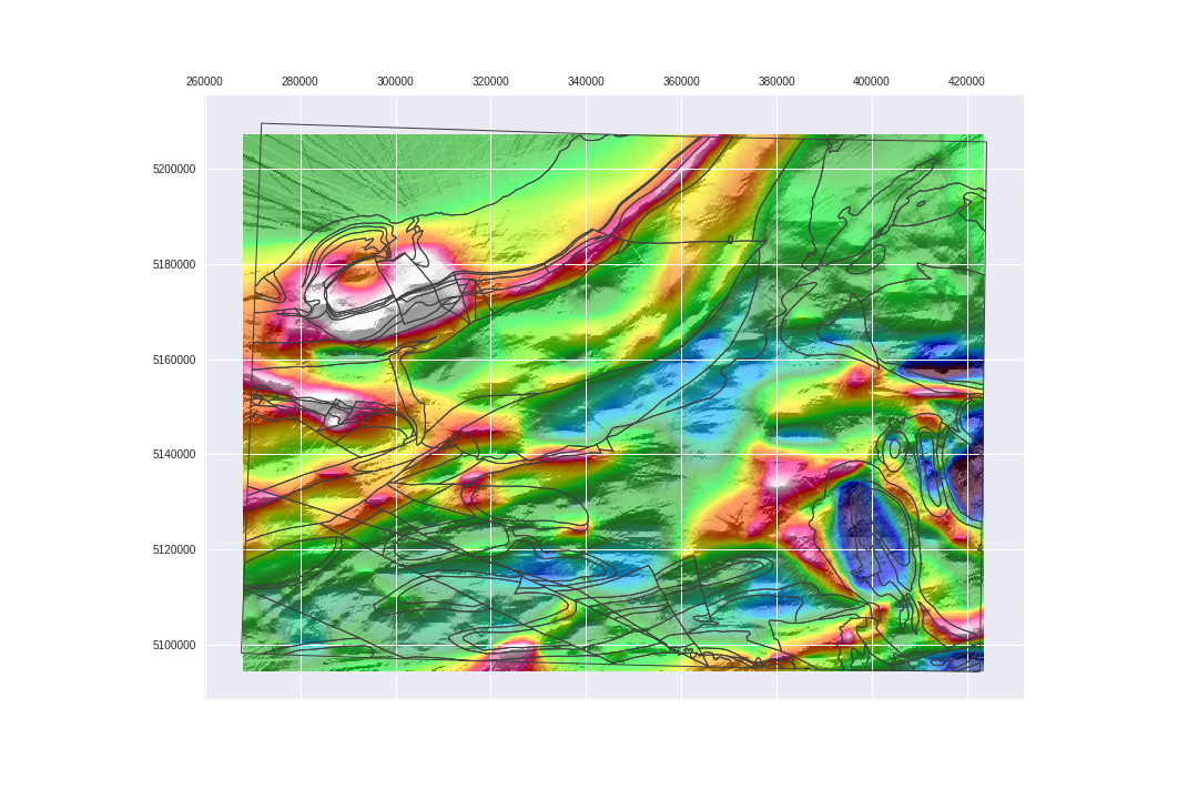
And, finally:

fig = plt.figure(figsize=(15, 10))
ax = fig.add_subplot(111)
ax.matshow(mag_TPOT, extent=extent, cmap=cmap, vmin=vmin, vmax=vmax)
ax.matshow(hillshade(mag_TPOT, 280, 25), extent=extent, cmap='Greys_r', alpha=.40)
geology.to_crs({'init': 'epsg:32616'}).plot(alpha=0, ax=ax, edgecolor='.25')
plt.savefig('images/7/12.png')

7-12

Let's save the arrays we just created.

np.save('./data/processed/arrays/mag_tpot_array', mag_TPOT)
np.save('./data/processed/arrays/mag_tpot_array_hs', hillshade(mag_TPOT, 280, 25))

Interested in using the code or want me to process your data?
Make contact: brunorpinho10@gmail.com

This post is PART 2 of the Integrating and Exploring series: