Download and Process DEMs in Python

This post is PART 3 of the Integrating and Exploring series:

Digital Elevation Models (DEMs) represents a 3D surface model of a terrain. They are how computers store and display topographic maps that, before, were only possible with handmade contours and extensive calculations. DEMs are probably essential for every topic in earth sciences. Understanding the processes that governs the surface of the earth, with today's technology, usually goes through the process of manipulating a DEM at some point. Also, we need a DEM to mask out data over the surface in our resource models or maybe quickly check what's the height on top of Aconcágua.

DEM can be in form of rasters or, a vector-based Triangulated Irregular Network (TIN).

In Python, recent modules and technics have made DEM rasters very simple to process and that's what we are going to integrate and explore in this post.

This is the PART 3 of a series of posts called Integrating & Exploring.

Area of Study

Fixed: was referencing wrong dataset

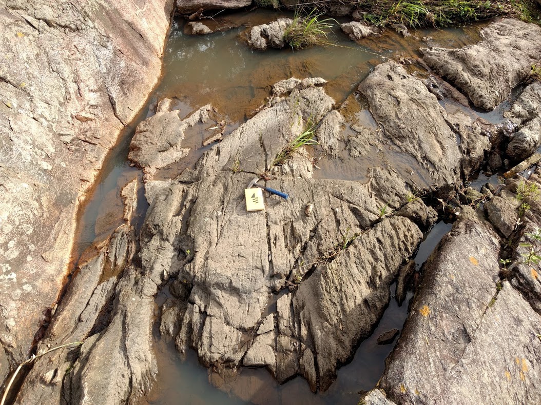
Iron River in Michigan, USA

I choose this specific area because of the presence of Geological, Geophysical and Geochemical data. It will be nice to explore!

Tutorial

We start by importing numpy for array creation and manipulation. The plt interface of matplotlib for plotting. seaborn for scientific graphs and geopandas that will be only used to import the area of study bounds.

import numpy as np
import matplotlib.pyplot as plt
import seaborn as sns
import geopandas as gpd
%matplotlib inline

Defining the bounds

Let's import the bounds of our Area of Study generated in PART 1.

bounds = gpd.read_file('./data/processed/area_of_study_bounds.gpkg').bounds

Check Geopandas output of .bounds:

bounds

	minx	miny	maxx	maxy
0	-90.000672	45.998852	-87.998534	46.999431

Split the list into separate variables.

west, south, east, north = bounds = bounds.loc[0]

Let's add 3" in every direction before we request the DEM to the server. This is important because, when we reproject the DEM from latlong to UTM, the data is translated, rotated and rescaled by an Affine matrix and we usually end up with missing information on the corners unless we select a bigger rectangle, and that's basically what we are doing here. Try skipping this line and continue the process.

west, south, east, north = bounds  = west - .05, south - .05, east + .05, north + .05

Download the data

A recent published packaged called elevation provide one-liners to download SRTM data. Let's use it.

import elevation

First, we define an absolute path to the dataset. (elevation didn't handle relative paths for me for some reason)

import os
dem_path = '/data/external/Iron_River_DEM.tif'
output = os.getcwd() + dem_path

Call the elevation method to download and clip the SRTM dataset according to the bounds we define above. This is just great stuff.

The product argument can be either 'SRTM3' for the 90m resolution dataset or 'SRTM1' for the 30m resolution. Since the grid we defined in PART 2 is 250m resolution let's get the DEM in 90m. The data is downloaded in form of raster to the path I defined above, which is ./data/external/Iron_River_DEM.tif.

elevation.clip(bounds=bounds, output=output, product='SRTM3')

Reproject to match the geophysics data

Now, we need to reproject the DEM to match the magnetics grid that was spatially predicted, in PART 2, using the UTM cartesian projection. To match, the projected DEM array must respect the following:

be in UTM zone 16 (EPSG:32616);
have a 250 meters spatial resolution;
have bounds equal to (xmin: 268000 m, xmax: 423500 m, ymin: 5094500 m, ymax: 5207000 m).

All of that is be done in one go using the amazing rasterio module. From the official docs:

Geographic information systems use GeoTIFF and other formats to organize and store gridded raster datasets such as satellite imagery and terrain models. Rasterio reads and writes these formats and provides a Python API based on Numpy N-dimensional arrays and GeoJSON.

Let's import everything we are going to use from rasterio.

from rasterio.transform import from_bounds, from_origin
from rasterio.warp import reproject, Resampling
import rasterio

rasterio method to read the raster we downloaded:

dem_raster = rasterio.open('.' + dem_path)

Extract the CRS information, along with the shape. The src_transform is the Affine transformation for the source georeferenced raster. We calculate it using the from_bounds function provided by rasterio. The bounds were processed above.

src_crs = dem_raster.crs
src_shape = src_height, src_width = dem_raster.shape
src_transform = from_bounds(west, south, east, north, src_width, src_height)
source = dem_raster.read(1)

Now that our source raster is ready. Let's go ahead and setup the destination array. Since the spatial resolution is a requirement, instead of from_bounds, it is just simpler to pass the top left coordinates (x: 268000.0, y: 5207000.0), the pixel size (250 m) and the shape of the destination arrays (height: 451, width 623). The coordinate system can be just a EPSG code:

dst_crs = {'init': 'EPSG:32616'}
dst_transform = from_origin(268000.0, 5207000.0, 250, 250)
dem_array = np.zeros((451, 623))
dem_array[:] = np.nan

Call reproject and it will do all the magic:

reproject(source,
          dem_array,
          src_transform=src_transform,
          src_crs=src_crs,
          dst_transform=dst_transform,
          dst_crs=dst_crs,
          resampling=Resampling.bilinear)

Visualization

The code below will check if pycpt is installed and will try to load a nice Colormap for Topographic visualization. If an error occurs, it will use the inverse of the matplotlib's Spectral Colormap.

try:
    import pycpt
    topocmap = pycpt.load.cmap_from_cptcity_url('wkp/schwarzwald/wiki-schwarzwald-cont.cpt')
except:
    topocmap = 'Spectral_r'

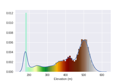
Define the minimum and maximum values for the Colormap.

vmin = 180
vmax = 575

Let's check how these values go:

ax = sns.distplot(dem_array.ravel(), axlabel='Elevation (m)')
ax = plt.gca()
_ = [patch.set_color(topocmap(plt.Normalize(vmin=vmin, vmax=vmax)(patch.xy[0]))) for patch in ax.patches]
_ = [patch.set_alpha(1) for patch in ax.patches]
ax.get_figure().savefig('images/8/1.png')

8-1

Define the extent for the topographic visualization:

extent = xmin, xmax, ymin, ymax = 268000.0, 423500.0, 5094500.0, 5207000.0

Let's add a hillshade layer.

This hillshade function is from the GeoExamples blog:

def hillshade(array, azimuth, angle_altitude):

    # Source: http://geoexamples.blogspot.com.br/2014/03/shaded-relief-images-using-gdal-python.html

    x, y = np.gradient(array)
    slope = np.pi/2. - np.arctan(np.sqrt(x*x + y*y))
    aspect = np.arctan2(-x, y)
    azimuthrad = azimuth*np.pi / 180.
    altituderad = angle_altitude*np.pi / 180.


    shaded = np.sin(altituderad) * np.sin(slope) \
     + np.cos(altituderad) * np.cos(slope) \
     * np.cos(azimuthrad - aspect)
    return 255*(shaded + 1)/2

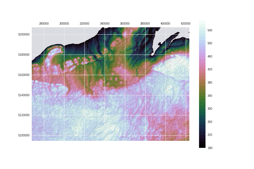
Finally:

fig = plt.figure(figsize=(12, 8))
ax = fig.add_subplot(111)
ax.matshow(hillshade(dem_array, 30, 30), extent=extent, cmap='Greys', alpha=.5, zorder=10)
cax = ax.contourf(dem_array, np.arange(vmin, vmax, 10),extent=extent, 
                  cmap=topocmap, vmin=vmin, vmax=vmax, origin='image')
fig.colorbar(cax, ax=ax)
fig.savefig('images/8/2.png')

8-2

Save the arrays:

np.save('./data/processed/arrays/dem_array', dem_array)
np.save('./data/processed/arrays/dem_array_hs', hillshade(dem_array, 280, 25))

UPDATE:

It was suggested by the geophysicist Matteo Nicolli to change the colormap for a more perceptual option like viridis. I admit that have never read about the important concepts of color visualizations before and here is a important quote from this matplotlib article (I recommend reading it):

For many applications, a perceptually uniform colormap is the best choice — one in which equal steps in data are perceived as equal steps in the color space. Researchers have found that the human brain perceives changes in the lightness parameter as changes in the data much better than, for example, changes in hue. Therefore, colormaps which have monotonically increasing lightness through the colormap will be better interpreted by the viewer.

I also recommend reading through Matteo's article about color visualization. Thanks Matteo!

Let's use the cubehelix colormap, which is designed with corrected luminosity, have a good color variation and is readily available in matplotlib.

fig = plt.figure(figsize=(12, 8))
ax = fig.add_subplot(111)
ax.matshow(hillshade(dem_array, 330, 30), extent=extent, cmap='Greys', alpha=.1, zorder=10)
cax = ax.contourf(dem_array, np.arange(vmin, vmax, 10),extent=extent, 
                  cmap='cubehelix', vmin=vmin, vmax=vmax, origin='image', zorder=0)
fig.colorbar(cax, ax=ax)
fig.savefig('images/8/3.png')

8-3

Now compare with the previous image. Isn't luminance exposing structures better?

!convert -delay 95 -loop 0 images/8/2.png images/8/3.png images/8/4.gif

8-1

This post is PART 3 of the Integrating and Exploring series: