Fast and Reliable Top of Atmosphere (TOA) calculations of Landsat-8 data in Python

This post is PART 5 of the Integrating and Exploring series:

In this tutorial, I will show how to extract reflectance information from Landsat-8 Level-1 Data Product images. If you don't know what I'm talking about:

Standard Landsat 8 data products provided by the USGS EROS Center consist of quantized and calibrated scaled Digital Numbers (DN) representing multispectral image data acquired by both the Operational Land Imager (OLI) and Thermal Infrared Sensor (TIRS). The products are delivered in 16-bit unsigned integer format and can be rescaled to the Top Of Atmosphere (TOA) reflectance and/or radiance using radiometric rescaling coefficients provided in the product metadata file (MTL file), as briefly described below. The MTL file also contains the thermal constants needed to convert TIRS data to the top of atmosphere brightness temperature.

In summary:

The DN is a scaled number of the measured values. We have ways to rescale the DN values into TOA values using coefficients that are found in the metadata files (MTL) that we usually download with the image files (TIF).
Top of Atmosphere (TOA) Reflectance and Brightness Temperature are what we use to study the earth surface material spectrum from multipectral satellite images. There are huge databases of known spectrums for a variety of materials measured in labs and convolved to different spectrometer and multispectral sensors. One good example is the USGS's Spectroscopy Lab, check their work.

Another important step in the processing of Landsat-8 files is to understand the possible artifacts. Please, read the Appendix A - Known Issues in the Data User Handbook. Knowing the possible artifacts will avoid headache during your analyses. When I hit one of those, I usually mask them out. Please, notice that some artifacts are not that simple to remove. For example, to remove striping from images we need to filter information out of the frequency domain using Fourier Transforms.

This is the PART 5 of a series of posts called Integrating & Exploring.

I downloaded the images in PART 4.

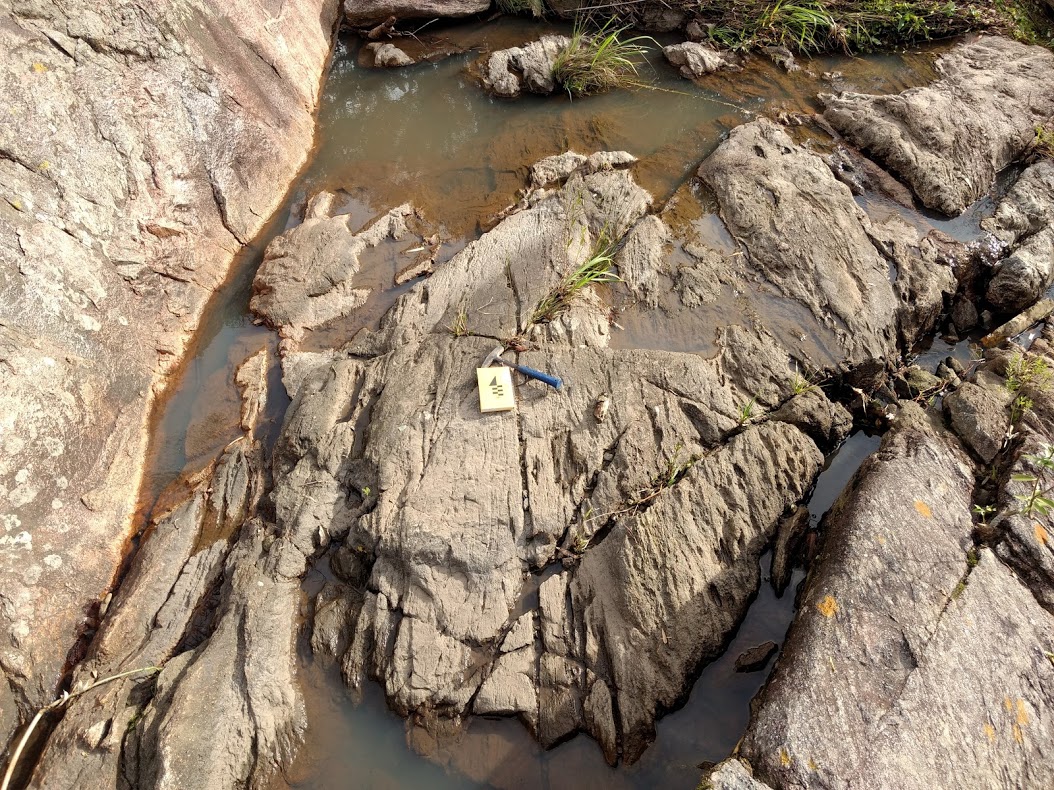
Area of Study

Iron River in Michigan, USA

Tutorial

Start by installing rio-toa for Top of Atmosphere (TOA) Landsat-8 calculations and rio-l8qa for Landsat 8 Quality Assessment (QA) processing. We will use the last one for a one-line solution cloud mask generator using the QA.

We will need to have rasterio installed for those.

!pip install rio-toa --quiet
!pip install rio-l8qa --quiet

Import glob for pathname searches.

os and shutil for file and path manipulations.

numpy and matplotlib for array manipulation and visualizations, respectively.

rasterio for raster reading/writing and simple manipulation functions.

reflectance from rio_toa to get reflectance out of Landsat-8 multispectral sensors measurements.

cartopy.crs for cartographic projections in matplotlib geopandas for geospatial data manipulations in pandas

tqdm_notebook for simple progress bars.

from glob import glob
import os
import shutil

import numpy as np
import matplotlib.pyplot as plt

import rasterio

from l8qa.qa import write_cloud_mask
from rio_toa import reflectance

from tqdm import tqdm_notebook

from cartopy import crs as ccrs
import geopandas as gpd

import warnings

warnings.simplefilter(action='ignore', category=FutureWarning)
warnings.simplefilter(action='ignore', category=UserWarning)

%matplotlib inline

Just like we did on the last post, setup some folder variables. SRC for source and DST for.. <hmm... I don't remember what DST stands for> destination.

SRC_LANDSAT_FOLDER = './data/external/Landsat8/'
DST_LANDSAT_FOLDER = './data/processed/Landsat8/'

Here, we define parameters for writing the raster files.

We want 0 values to be nodata, deflate compression (more info here and here), predict is a parameter for the deflate compression.

processes is an integer, the number of CPUs processing.

rescale_factor is very well explained in this rio-toa topic:

Note that we need to rescale post-TOA tifs to 55,000 instead of 216 because USGS Landsat 8 products are delivered as 16-bit images but are actually scaled to 55,000 grey levels.

creation_options = {'nodata': 0,
                    'compress': 'deflate',
                    'predict': 2}

processes = 4
rescale_factor = 55000
dtype = 'uint16'

Optional requirement: pip install tqdm

The cell below will, initially, use glob to find all Landsat-8 Image folders located in the SRC_LANDSAT_FOLDER. Then, for each folder it will make a folder with the same name in the DST_LANDSAT_FOLDER.

After that, it will use glob again to find the metadata (MTL.txt) and the Quality Assessment (QA) files.

Then, process the reflectance from bands 1 to 9.

# Use `glob` to find all Landsat-8 Image folders.
l8_images = glob(os.path.join(SRC_LANDSAT_FOLDER, 'L*/'))

# Here we will set up `tqdm` progress bars to keep track of our processing. 
# (This is an optional step, I like progress bars)
pbar_1st_loop = tqdm_notebook(l8_images, desc='Folder')

for src_folder in pbar_1st_loop:
    # Get the name of the current folder
    folder = os.path.split(src_folder[:-1])[-1]

    # Make a folder with the same name in the `DST_LANDSAT_FOLDER`.
    dst_folder = os.path.join(DST_LANDSAT_FOLDER, folder)
    os.makedirs(dst_folder, exist_ok=True)

    # Use `glob` again to find the metadata (`MTL.txt`) and the Quality Assessment (`QA`) files
    src_mtl = glob(os.path.join(src_folder, '*MTL*'))[0]
    src_qa = glob(os.path.join(src_folder, '*QA*'))[0]

    # Here we will create the cloudmask
    # Read the source QA into an rasterio object.
    with rasterio.open(src_qa) as qa_raster:
        # Update the raster profile to use 0 as 'nodata'
        profile = qa_raster.profile
        profile.update(nodata=0)

        #Call `write_cloud_mask` to create a mask where the QA points to clouds.
        write_cloud_mask(qa_raster.read(1), profile, os.path.join(dst_folder, 'cloudmask.TIF'))

    # Set up the second loop. For bands 1 to 9 in this image.
    pbar_2nd_loop = tqdm_notebook(range(1, 10), desc='Band')

    # Iterate bands 1 to 0 using the tqdm_notebook object defined above
    for band in pbar_2nd_loop: 

        # Use glob to find the current band GeoTiff in this image.
        src_path = glob(os.path.join(src_folder, '*B{}.TIF'.format(band)))

        dst_path = os.path.join(dst_folder, 'TOA_B{}.TIF'.format(band))

        # Writing reflectance takes a bit to process, so if it crashes during the processing,
        # this code skips the ones that were already processed.
        if not os.path.exists(dst_path): 

            # Use the `rio-toa` module for reflectance.
            reflectance.calculate_landsat_reflectance(src_path, src_mtl, 
                                                      dst_path,
                                                      rescale_factor=rescale_factor, 
                                                      creation_options=creation_options,
                                                      bands=[band], dst_dtype=dtype,
                                                      processes=processes, pixel_sunangle=True)

    # Just copy the metadata from source to destination in case we need it in the future.
    shutil.copy(src_mtl, os.path.join(dst_folder, 'MTL.txt'))

Notice that without downsampling or clipping, we will take so much time to process. In my old machine, it took ~2 min per image. One could downsample the images first with rasterio's reproject to decrease the processing time. However, I didn't do it in this post because I want to explore all the data (more info after the plot).

Let's check the reflectance for Band 5. I'm setting up two matplotlib figures. One for the rasters and another one for distribution plot.

from matplotlib.cm import viridis as cmap
import matplotlib.patheffects as pe

bounds = gpd.read_file('./data/processed/area_of_study_bounds.gpkg')

xmin, xmax, ymin, ymax = [], [], [], []

for image_path in glob(os.path.join(DST_LANDSAT_FOLDER, '*/*B5.TIF')):
    with rasterio.open(image_path) as src_raster:
        xmin.append(src_raster.bounds.left)
        xmax.append(src_raster.bounds.right)        
        ymin.append(src_raster.bounds.bottom)        
        ymax.append(src_raster.bounds.top)       

fig, ax = plt.subplots(1, 1, figsize=(20, 15), subplot_kw={'projection': ccrs.UTM(16)})
hist_fig, hist_axes = plt.subplots(1, 4, figsize=(20, 5), sharey=True)

ax.set_extent([min(xmin), max(xmax), min(ymin), max(ymax)], ccrs.UTM(16))

bounds.plot(ax=ax, transform=ccrs.PlateCarree())

for hax, image_path in zip(hist_axes.ravel(), glob(os.path.join(DST_LANDSAT_FOLDER, '*/*B5.TIF'))):

    pr = image_path.split('/')[-2].split('_')[2]
    path_row = 'P: {}  R: {}'.format(pr[:3], pr[3:])

    with rasterio.open(image_path) as src_raster:

        extent = [src_raster.bounds[i] for i in [0, 2, 1, 3]]  

        dst_transform = rasterio.transform.from_origin(src_raster.bounds.left, src_raster.bounds.top, 250, 250)

        width = np.ceil((src_raster.bounds.right - src_raster.bounds.left) / 250.).astype('uint')
        height = np.ceil((src_raster.bounds.top - src_raster.bounds.bottom) / 250.).astype('uint')

        dst = np.zeros((height, width))

        rasterio.warp.reproject(src_raster.read(1), dst, 
                  src_transform=src_raster.transform, 
                  dst_transform=dst_transform,
                  resampling=rasterio.warp.Resampling.nearest)

        cax = ax.matshow(np.ma.masked_equal(dst, 0) / 550.0, cmap=cmap,
                   extent=extent, transform=ccrs.UTM(16),
                   vmin=10, vmax=40)

        t = ax.text((src_raster.bounds.right + src_raster.bounds.left) / 2, 
                    (src_raster.bounds.top + src_raster.bounds.bottom) / 2, 
                    path_row,
                    transform=ccrs.UTM(16), 
                    fontsize=20, ha='center', va='top', color='.1', 
                    path_effects=[pe.withStroke(linewidth=3, foreground=".9")])

        sns.distplot(dst.ravel() / 550.0, ax=hax, axlabel='Reflectance (%)', kde=False, norm_hist=True)
        hax.set_title(path_row, fontsize=13)
        hax.set_xlim(0,100); hax.set_ylim(0,.1)

        [patch.set_color(cmap(plt.Normalize(vmin=10, vmax=40)(patch.xy[0]))) for patch in hax.patches]
        [patch.set_alpha(1) for patch in hax.patches]

        del dst

fig.colorbar(cax, ax=ax, label='Reflectance (%)')
fig.savefig('./images/11/band-5.png', transparent=True, bbox_inches='tight', pad_inches=0)
hist_fig.savefig('./images/11/hist-band-5.png', transparent=True, bbox_inches='tight', pad_inches=0)

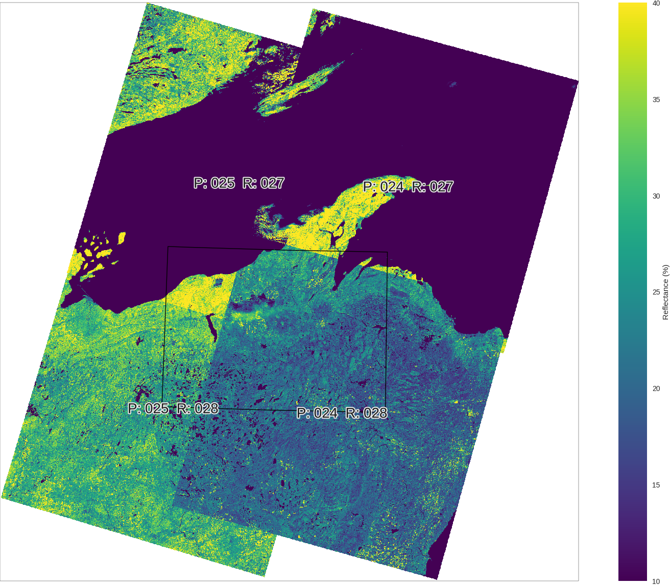
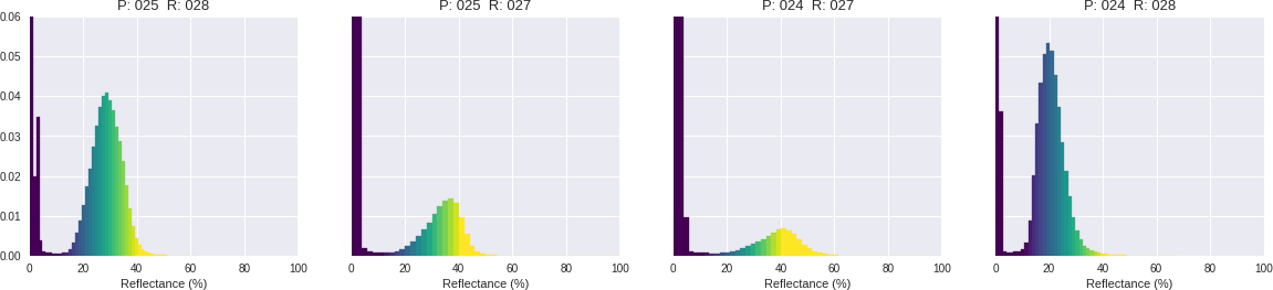
This is a very common situation when we are combining several images into one. Their histograms don't quite match each other even though they are are the same wavelength measuring the same structures on earth (where they overlap). This is probably because these measurements are very sensitive to number of natural aspects, like light sources, hour of the day, etc. I want to explore solutions for mosaicking these images band by band using ML. (Depending on how it goes, I will post it here.)

There's not much python advanced mosaicking options out there is it? Please, contribute !

This post is PART 5 of the Integrating and Exploring series: