Processing Shapefiles of Lithological Units

This post is PART 1 of the Integrating and Exploring series:

This is the PART 1 of a series of posts called Integrating & Exploring.

In these posts, I will do all the preprocessing that I normally do when I work with multiple data sources like Geological Maps, Geophysics and Geochemistry.

The preprocessed data will be used in future posts where I will explore topics like Geostatistics, Machine Learning, Data Analysis and more.

To start, I will present the data and the area that I chose to process. For PART 1 I will show some GIS technics using GeoPandas and Folium.

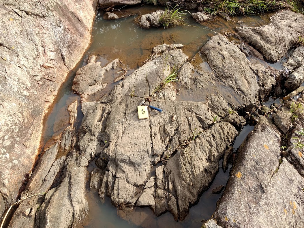
Area of Study

Fixed: was referencing wrong dataset

Iron River in Michigan, USA

I choose this specific area because of the presence of Geological, Geophysical and Geochemical data. It will be nice to explore!

Data

All data was downloaded from the USGS - Mineral Resources Online Spatial Data. The data is composed by:

one Geophysics surveys (Magnetic anomaly and Radiometric - in .xyz);
two Geological Maps (WI and MI, USA - in .shp);

Geology

Michigan geologic map data : A GIS database of geologic units and structural features in Michigan, with lithology, age, data structure, and format written and arranged just like the other states.

Geophysics

Title: Airborne geophysical survey: Iron River 1° x 2° Quadrangle

Publication_Date: 2009

Geospatial_Data_Presentation_Form: tabular digital data

Online_Linkage: https://mrdata.usgs.gov/magnetic/show-survey.php?id=NURE-164

Metadata: https://mrdata.usgs.gov/geophysics/surveys/NURE/iron_river/iron_river_meta.html

Beginning Flight Date: 1977 / 04 / 25

Survey height: 400 ft

Flight-line spacing: 3 miles

Soil Geochemistry

I downloaded a big chunk of the USGS's National Geochemical Database - Soil around the Area of Interest in CSV format.

Location

We are going to use the geophysics to get the bounds of the area and start with the location. So let's import some modules first:

import numpy as np
import pandas as pd
import geopandas as gpd
import pyproj
import folium
from shapely import geometry
import matplotlib.pyplot as plt

%matplotlib inline

From the Gephysics Metadata I copied the header for the .xyz file.

With the header, we can identify which columns are the latitude and longitude.

I pasted the header as a space delimited string. Now I have to use a string method to .split the data and end up with a list.

column_names = 'line fid time day year latitude longitude radalt totmag resmag diurnal geology resmagCM4'.split(' ') 
print column_names

['line', 'fid', 'time', 'day', 'year', 'latitude', 'longitude', 'radalt', 'totmag', 'resmag', 'diurnal', 'geology', 'resmagCM4']

Now, when I import the data into a pandas DataFrame (DF), I can identify the columns that I want to use with the usecols argument. Also, the delim_whitespace tells pandas that this is a whitespace delimited text file:

Specifies whether or not whitespace (e.g. ' ' or ' ') will be used as the sep. Equivalent to setting sep='\s+'. If this option is set to True, nothing should be passed in for the delimiter parameter.

mag_data = pd.read_csv('./data/raw/Geophysics/iron_river_mag.xyz.gz', 
                       delim_whitespace=True, names=column_names, usecols=['latitude', 'longitude', 'totmag'])
mag_data.head() # This shows the first 5 entries of the DF.

	latitude	longitude	totmag
0	46.0237	-89.9960	59280.2
1	46.0237	-89.9950	59283.0
2	46.0237	-89.9944	59283.8
3	46.0237	-89.9934	59281.0
4	46.0237	-89.9928	59276.5

From the metadata we have that the geophysics data is referenced to latlong (NAD27) datum. Let's use pyproj to transform it to both latlong (WGS84) and UTM zone 16 (WGS84).

# North American Datum 1927
p1 = pyproj.Proj(proj='latlong', datum='NAD27')
# WGS84 Latlong
p2 = pyproj.Proj(proj='latlong', datum='WGS84')
# WGS84 UTM Zone 16
p3 = pyproj.Proj(proj='utm', zone=16, datum='WGS84')
mag_data['long_wgs84'], mag_data['lat_wgs84'] = pyproj.transform(p1, p2, 
                                                            mag_data.longitude.values, 
                                                            mag_data.latitude.values)
mag_data['E_utm'], mag_data['N_utm'] = pyproj.transform(p1, p3,
                                                        mag_data.longitude.values,
                                                        mag_data.latitude.values)

GeoPandas is a package to manipulate geospatial files the same way you manipulate pandas DataFrames. From the docs:

GeoPandas is an open source project to make working with geospatial data in python easier. GeoPandas extends the datatypes used by pandas to allow spatial operations on geometric types. Geometric operations are performed by shapely. Geopandas further depends on fiona for file access and descartes and matplotlib for plotting.

To transform our pandas DataFrame into a geopandas GeoDataFrame we have to create a geometry columns that cointains a shapely.geometry object for each entry. Let's iterate through the rows and transform longitude and latitude values into a list filled with Point objects for each entry. Then, we add it into the DataFrame:

mag_data['geometry'] = [geometry.Point(x, y) for x, y in zip(mag_data['long_wgs84'], mag_data['lat_wgs84'])]

Pass the DataFrame to a GeoDataFrame object indicating which one is the geometry columns and the CRS (Coordinate Reference System):

mag_data = gpd.GeoDataFrame(mag_data, geometry='geometry', crs="+init=epsg:4326")

Let's save it to a CSV file to reuse it when we start processing the Aeromagnetic Data:

mag_data.to_csv('./data/processed/mag.csv')

Let's check the first 3 entries:

mag_data.head(3)

	latitude	longitude	totmag	long_wgs84	lat_wgs84	E_utm	N_utm	geometry
0	46.0237	-89.9960	59280.2	-89.996159	46.023649	268103.008274	5.101040e+06	POINT (-89.99615875516027 46.02364873764436)
1	46.0237	-89.9950	59283.0	-89.995159	46.023649	268180.405926	5.101037e+06	POINT (-89.99515872940462 46.02364874420012)
2	46.0237	-89.9944	59283.8	-89.994559	46.023649	268226.844518	5.101036e+06	POINT (-89.99455871395124 46.02364874813357)

.envelope is a shapely method to get the bounding rectangle of all the points in the geometry.

multipoints = geometry.MultiPoint(mag_data['geometry'])
bounds = multipoints.envelope

Let's save the bounds for the next parts of Integrating & Exploring.

gpd.GeoSeries(bounds).to_file('./data/processed/area_of_study_bounds.gpkg', 'GPKG')

Let's get the coordinates of the .boundary of the bounds.

coords = np.vstack(bounds.boundary.coords.xy)

Calculate the mean of the coordinates using numpy to center the location map on this.

map_center = list(coords.mean(1))[::-1]

Folium is a nice module to quickly visualize maps, in Python, using Leaflet.js. You don't even need to bother with JavaScript.

Explore the Folium's Gallery

Here, we create a map and add a PolyLine using the coordinates we just calculated. This is the limits of our Area of Study.

map_center

[46.399083592610125, -89.199816959726689]

m = folium.Map(location=map_center, zoom_start=8, control_scale=True)
folium.PolyLine(coords[::-1].T).add_to(m)
folium.LatLngPopup().add_to(m)
m

Geology

For this tutorial I downloaded two files with geological spatial data. These two files are the Geology of Michigan and Wisconsin, two states of the United States. Our Area of Study is on the border of these two states.

GeoPandas reads shapefiles straight into GeoDataFrames with the .read_file method.

Let's import both files:

geology_MI = gpd.read_file('./data/raw/Geology/MIgeol_dd/migeol_poly_dd.shp')
geology_WI = gpd.read_file('./data/raw/Geology/WIgeol_dd/wigeol_poly_dd.shp')

Now we use .append to append the two GeoDataFrames into one.

geology = geology_MI.append(geology_WI, ignore_index=True)
del(geology_MI)
del(geology_WI)

Let's check a random entry and see what interests us.

geology.loc[800]

AREA                                                0.000546392
MIGEOL_DD1                                                  NaN
MIGEOL_DD_                                                  NaN
ORIG_LABEL                                                  Agn
PERIMETER                                              0.225196
ROCKTYPE1                                                gneiss
ROCKTYPE2                                           amphibolite
SGMC_LABEL                                                Agn;0
SOURCE                                                    WI003
UNIT_AGE                                                Archean
UNIT_LINK                                               WIAgn;0
WIGEOL_DD1                                                  329
WIGEOL_DD_                                                  110
geometry      POLYGON ((-89.28126080384193 46.17530270637592...
Name: 800, dtype: object

Alright, now let's drop everything and keep only the geometry, the rock types and the unit link.

geology = geology.loc[:, ['geometry', 'ROCKTYPE1', 'ROCKTYPE2', 'UNIT_LINK']]

geology.head(3)

	geometry	ROCKTYPE1	ROCKTYPE2	UNIT_LINK
0	POLYGON ((-89.4831513887011 48.01386246799924,...	water		MIwater;0
1	POLYGON ((-88.36638683756532 48.22117182372271...	basalt	andesite	MIYplv;0
2	POLYGON ((-88.47487656107728 48.17241499899792...	basalt	andesite	MIYplv;0

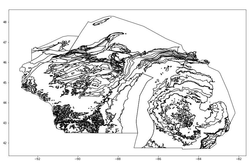
Let's use GeoPandas plot method to see what we got so far:

ax = geology.plot(facecolor='w', figsize=(12,8))
fig = ax.figure; fig.tight_layout()
fig.savefig('images/6/1.png')

6-1

Next, we are going to use shapely to check if each polygon intersects the bounds of our Area of Study. If it DOES intersect, we are going to clip it using the .intersection method of the polygon according to the bounds and update the entry. If it DOES NOT intersect, we add it's index to the drop list and drop it after the loop.

todrop = []

# Start the iteration:
for i, row in geology.iterrows():
    # Check if intersect with the bounds
    if row.geometry.intersects(bounds):
        # Clip using .intersection and update the entry.
        geology.set_value(i, 'geometry', row.geometry.intersection(bounds))
    else:
        todrop.append(i)

# Drop entries that don't intersect with the bounds
geology.drop(geology.index[todrop], inplace=True)

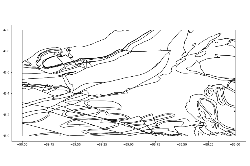
Let's see our new GeoDataFrame:

ax = geology.plot(facecolor='w', figsize=(12,8))
fig = ax.figure; fig.tight_layout()
fig.savefig('images/6/2.png')

6-2

Applying colors

Good, now we are going to apply the USGS's lithological color table to our geological map.

First, we need to change all the "meta-basalt" entries to "metabasalt", because that's how it is in the color table.

geology.loc[geology['ROCKTYPE1'].str.contains('meta-basalt'), 'ROCKTYPE1'] = 'metabasalt'

Import the color system into a DataFrame and use the column text (lowercase) as index.

colors = pd.read_csv('./data/raw/Geology/color_data.txt', delimiter='\t')
colors.index = colors.text.str.lower()
colors.replace('-', '')
colors.head()

	code	r	g	b	text
text
unconsolidated material	1	253	244	63	Unconsolidated material
alluvium	1.1	255	255	137	Alluvium
silt	1.10	255	211	69	Silt
sand	1.11	255	203	35	Sand
flood plain	1.1.1	255	255	213	Flood plain

In order to use folium with colors we need a new column joining the r,g,b values into a different format. Could be the hex format (ex. '#ffffff') or the svg format ('rgba(r,g,b,a)').

We do both with a lambda function and the DataFrame.apply method.

Python lambda function:

Small anonymous functions can be created with the lambda keyword. This function returns the sum of its two arguments: lambda a, b: a+b. Lambda functions can be used wherever function objects are required. They are syntactically restricted to a single expression. Semantically, they are just syntactic sugar for a normal function definition. Like nested function definitions, lambda functions can reference variables from the containing scope:

pandas DataFrame.apply method:

Applies function along input axis of DataFrame.

Objects passed to functions are Series objects having index either the DataFrame’s index (axis=0) or the columns (axis=1). Return type depends on whether passed function aggregates, or the reduce argument if the DataFrame is empty.

from matplotlib.colors import to_hex

colors['rgba'] = colors.apply(lambda x:'rgba(%s,%s,%s,%s)' % (x['r'],x['g'],x['b'], 255), axis=1)
colors['hex'] = colors.apply(lambda x: to_hex(np.asarray([x['r'],x['g'],x['b'],255]) / 255.0), axis=1)

colors.head()

	code	r	g	b	text	rgba	hex
text
unconsolidated material	1	253	244	63	Unconsolidated material	rgba(253,244,63,255)	#fdf43f
alluvium	1.1	255	255	137	Alluvium	rgba(255,255,137,255)	#ffff89
silt	1.10	255	211	69	Silt	rgba(255,211,69,255)	#ffd345
sand	1.11	255	203	35	Sand	rgba(255,203,35,255)	#ffcb23
flood plain	1.1.1	255	255	213	Flood plain	rgba(255,255,213,255)	#ffffd5

We have multiple Polygons for same ROCK TYPES. Let's separate the geology by groups of ROCKTYPE1 using the DataFrame.groupy method:

rock_group = geology.groupby('ROCKTYPE1')

Check the group names:

print ' - '.join(rock_group.groups)

limestone - graywacke - amphibolite - gabbro - sandstone - siltstone - arkose - schist - granite - metamorphic rock - quartzite - mafic metavolcanic rock - iron formation - slate - basalt - water - syenite - andesite - conglomerate - metasedimentary rock - metabasalt - rhyolite - gneiss - mica schist - metavolcanic rock

Create a new folium map and, for each rock_group, add the entries of that group to the map using the folium.GeoJson method.

This method imports GeoDataFrames straight into the maps.

[GeoJSON](http://geojson.org/) is a format for spatial files and all `GeoDataFrames` have a simple method to be converted to GeoJSON. This is why it just works.

To add the colors, pass a lambda function containing the style for each entry to the argument style_function in the folium.GeoJson method. Also, for each GeoJSON object we a Popup as child with the .add_child method.

m = folium.Map(location=map_center, zoom_start=8, height='100%', control_scale=True)
fg = folium.FeatureGroup(name='Geology').add_to(m)

for rock in rock_group.groups.keys():
    rock_df = geology.loc[geology.ROCKTYPE1 == rock]
    style_function = lambda x: {'fillColor': colors.loc[x['properties']['ROCKTYPE1']]['hex'],
                                'opacity': 0, 
                                'fillOpacity': .85,
                               }
    g = folium.GeoJson(rock_df, style_function=style_function, name=rock.title())
    g.add_child(folium.Popup(rock.title()))
    fg.add_child(g)

folium.LayerControl().add_to(m)
m

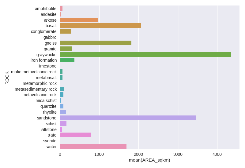
To calculate the area for each rocktype group.

First calculate the area for each Polygon in the GeoDataFrame. In order to get the area in sq. meters, transform the polygons to UTM system. Then call the .area method and divide by 10⁶ for sq. kilometers.

geology['AREA_sqkm'] = geology.to_crs({'init': 'epsg:32616'}).area / 10**6

Get the sum for all properties of the group:

rock_group_sum = rock_group.sum()
rock_group_sum['ROCK'] = rock_group_sum.index

rock_group_sum.head()

	AREA_sqkm	ROCK
ROCKTYPE1
amphibolite	68.142404	amphibolite
andesite	21.556282	andesite
arkose	983.557830	arkose
basalt	2068.717212	basalt
conglomerate	278.786114	conglomerate

Then, use seaborn for drawing a attractive graphic.

import seaborn as sns

ax = sns.barplot(y='ROCK', x='AREA_sqkm', data=rock_group_sum)
fig = ax.get_figure(); fig.tight_layout()
fig.savefig('images/6/3.png', dpi=100)

6-3

Another useful programming tip, in Python, is to request all about a specific Rock Unit (UNIT_LINK) to a online database.

Let's choose a random Unit:

geology.loc[51]

geometry     POLYGON ((-89.63811455333519 46.78150151277683...
ROCKTYPE1                                         conglomerate
ROCKTYPE2                                            sandstone
UNIT_LINK                                               MIYc;0
AREA_sqkm                                              180.851
Name: 51, dtype: object

So we have to request using the UNIT_LINK MIYc;0.

For the USGS database:

import requests

response = requests.request('GET', 'https://mrdata.usgs.gov/geology/state/json/{}'.format('MIYc;0')).json()

Now just explore the response.

response.keys()

[u'unit_name',
 u'geo',
 u'unitdesc',
 u'state',
 u'rocktype',
 u'unit_link',
 u'lith',
 u'unit_com',
 u'orig_label',
 u'ref',
 u'prov_no',
 u'unit_age']

print response['unitdesc']

Copper Harbor Conglomerate - Red lithic conglomerate and sandstone; mafic to felsic volcanic flows similar to those of the unnamed formation (unit Yu) are interlayered with the sedimentary rocks.

print response['unit_age']

Middle Proterozoic

Why not create a last iterative map with rock description?

This may take a while to process because we are requesting all units in the Area of Study to the USGS server.

m = folium.Map(location=map_center, zoom_start=8, height='100%', control_scale=True)
fg = folium.FeatureGroup(name='Geology').add_to(m)

for unit in geology.groupby('UNIT_LINK').groups.keys():
    unit_df = geology.loc[geology.UNIT_LINK == unit]
    description = requests.request(
        'GET', 'https://mrdata.usgs.gov/geology/state/json/{}'.format(unit)).json()['unitdesc']
    style_function = lambda x: {'fillColor': colors.loc[x['properties']['ROCKTYPE1']]['hex'],
                                'opacity': 0, 
                                'fillOpacity': .85,
                               }
    g = folium.GeoJson(unit_df, style_function=style_function)
    g.add_child(folium.Popup(description))
    fg.add_child(g)

folium.LayerControl().add_to(m)
m

Save the Geology shapefile for the next parts of Integrating & Exploring.

geology.to_file('./data/processed/geology/geology.shp')

Sources

Michigan geologic map data

Milstein, Randall L. (compiler), 1987, Bedrock geology of southern Michigan: Geological Survey Division, Michigan Dept. of Natural Resources, scale= 1:500,000

Reed, Robert C., and Daniels, Jennifer (compilers), 1987, Bedrock geology of northern Michigan: Geological Survey Division, Michigan Dept. of Natural Resources, scale= 1:500,000

Sims, P.K., 1992, Geologic map of Precambrian rocks, southern Lake Superior region, Wisconsin and northern Michigan: U.S. Geological Survey Miscellaneous Investigations Map I-2185, scale= 1:500,000

Cannon, W.F., Kress, T.H., Sutphin, D.M., Morey, G.B., Meints, Joyce, and Barber-Delach, Robert, 1997, Digital Geologic Map and mineral deposits of the Lake Superior Region, Minnesota, Wisconsin, Michigan: USGS Open-File Report 97-455 (version 3, Nov. 1999), on-line only

Wisconsin geologic map data

Mudrey, M.G., Jr., Brown, B.A., and Greenberg, J.K., 1982, Bedrock Geologic Map of Wisconsin: University of Wisconsin-Extension, Geological and Natural History Survey, scale= 1:1,000,000

Sims, P.K., 1992, Geologic map of Precambrian rocks, southern Lake Superior region, Wisconsin and northern Michigan: U.S. Geological Survey Miscellaneous Investigations Map I-2185, scale= 1:500,000

Cannon, W.F., Kress, T.H., Sutphin, D.M., Morey, G.B., Meints, Joyce, and Barber-Delach, Robert, 1997, Digital Geologic Map and mineral deposits of the Lake Superior Region, Minnesota, Wisconsin, Michigan: USGS Open-File Report 97-455 (version 3, Nov. 1999), on-line only

USGS Geologic Names Lexicon (GEOLEX)

Airbourne Geophysics of the Iron Mtn

U.S. Department of Energy, U.S. Geological Survey, Department of Interior and the National Geophysical Data Center, NOAA, 2009, Airborne geophysical survey: Iron River 1° x 2° Quadrangle:.
Sources

If you are making use of our methods, please consider donating. The button is at the bottom of the page.

This post is PART 1 of the Integrating and Exploring series: